Semi-sparsity for Smoothing Filters

Abstract:

We propose an interesting semi-sparsity smoothing algorithm based on a novel sparsity-inducing optimization framework. This method is derived from the multiple observations, that is, semi-sparsity prior knowledge is more universally applicable, especially in areas where sparsity is not fully admitted, such as polynomial-smoothing surfaces. We illustrate that this semi-sparsity can be identified into a generalized $L_0$-norm minimization in higher-order gradient domains, thereby giving rise to a new “feature-aware” filtering method with a powerful simultaneous-fitting ability in both sparse features (singularities and sharpening edges) and non-sparse regions (polynomial-smoothing surfaces). Notice that a direct solver is always unavailable due to the non-convexity and combinatorial nature of $L_0$-norm minimization. Instead, we solve the model based on an efficient half-quadratic splitting minimization with fast Fourier transforms (FFTs) for acceleration. We finally demonstrate its versatility and many benefits to a series of signal/image processing and computer vision applications.

Introduction

Filtering techniques, especially the feature-preserving algorithms, have been used as basic tools in signal/image processing fields. This favor is largely due to the fact that a variety of natural signals and visual clues (surfaces, depth, color, and lighting, etc.) tend to spatially have piece-wise constant or smoothing property, between which a minority of corner points and edges — known as sparse singularities or features formed by discontinuous boundaries convey an important proportion of useful information. On the basis of this prior knowledge, many filtering methods are promoted to have “feature-preserving” properties to preserve the sparse features while decoupling the local details or unexpected noise. The prevailing use of “feature-preserving” filtering methods is also found in many applications, including image denoise, tone mapping, and high dynamic range (HDR) image compression, details enhancement, stylization, and so on.

In the paper, we propose a semi-sparse minimization scheme for a type of smoothing filters. This new model is motivated by the sparsity-inducing priors used in recent cutting-edge filtering methods. It turns out that sparsity priors could help to pursue piece-wise constant filtering results and they are particularly suitable for preserving the sparse features (singularities and edges) existing in signals/images. Nevertheless, it worthy notice that sparsity priors may fail in the regions coexisting sparse features and polynomial smoothing surfaces (See Fig. 1). This failure, as interpreted hereafter, is largely due to the fact that sparse priors may be no longer fully admitted in the polynomial-smoothing surfaces, thereby leading to strong stair-case artifacts when imposing sparse regularization in these regions. In contrast, we illustrate that semi-sparsity priors enjoy more favorable properties in simultaneously fitting both sharpening singularities and polynomial-smoothing surfaces. This major difference leads to a new smoothing behavior that helps to alleviate the drawbacks of many existing filtering methods. We will interpret the semi-sparsity model and show the universal applicability of semi-sparsity prior knowledge for natural images.

Observations:

The $L_0$ norm counts the number of its non-zero entries, which directly measures the degree of sparsity of the vector. As a metric, it has been proved to be capable of capturing the singularities and discontinues of signals. In signal and image processing, a corresponding $L_0$ regularization is always a favorable and powerful mathematical tool to formulate the sparsity-induced priors. 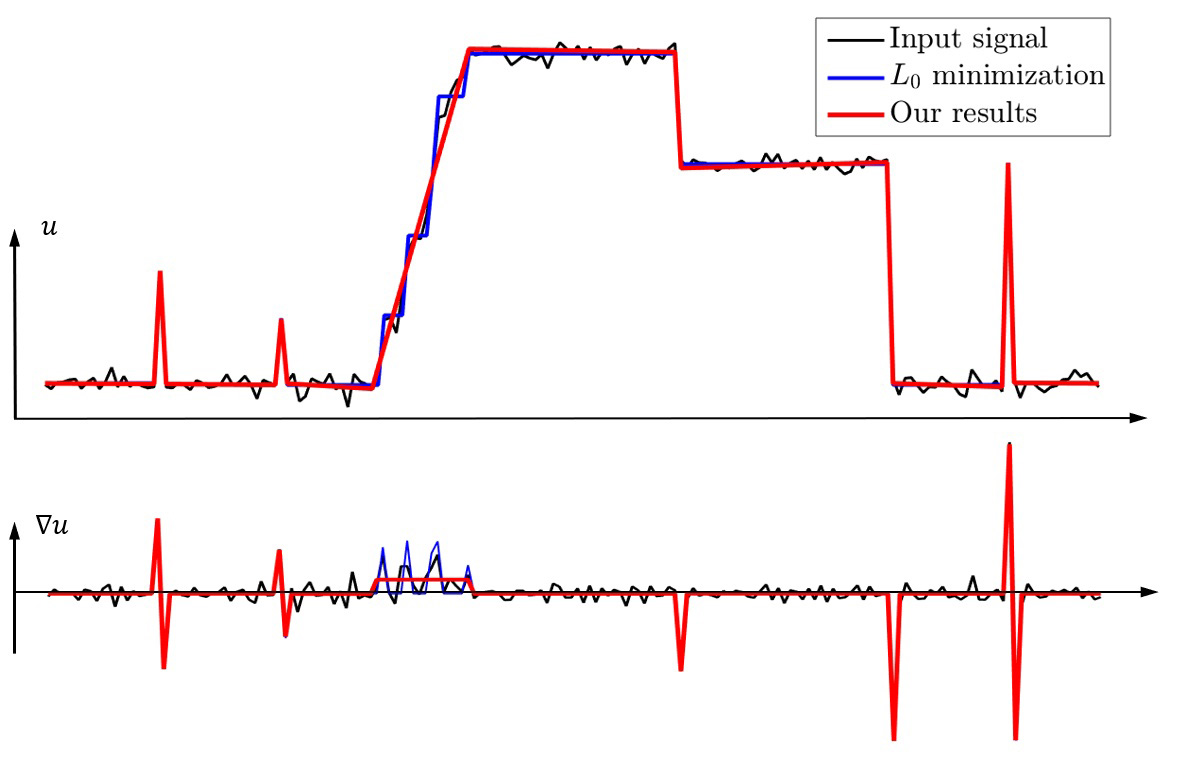It has been used in a huge amount of existing works, including sparse signal/image recovering sparse representation and compressed sensing and so on.

Figure 1. An example of 1D signal smoothing. This signal is composed of the spikes (singularities), sharp edges, and slope line (or, polynomial surface). It is clear that $L_0$ gradient minimizationpreserves spikes and sharp edges successfully but produces stair-case artifacts within the slope region (\textcolor{blue}{blue line}). In contrast, our model attains much better fitting (filtering) results in polynomial surfaces with comparable results in spikes and sharp edges ( red line ).

As interpreted in Fig. 1, the non-zero elements of gradient $\nabla u$ is not fully sparse but are densely distributed in some region. We say $u$ is a so-called semi-sparse signal in gradient domains in this case. On the other hand, it is easy to verify that the second order gradient ${\Delta u}$ is sparse. Without loss of generality, we define that $u$ is a semi-sparse signal, if the higher-order gradients ${\nabla}^{n-1} u$ and ${\nabla}^{n} u$ satisfy,

\[\begin{equation}\label{eq:4} \begin{aligned} \begin{cases} & {\left\Vert \nabla^{n} u\right\Vert}_0 < M,\\ &{\left\Vert \nabla^{n-1} u\right\Vert}_0 > N. \end{cases} \end{aligned} \end{equation}\]

where, ${\nabla}^{n}$ is a $n$-th (partial) differential operator, and $M, N$ are some appropriate natural number with ${M\ll N}$. The idea of Eq. (4) is easy to understand, that is, the energy of ${\nabla}^{n} u$ is much smaller than that of ${\nabla}^{n-1} u$. Intuitively, this happens if and only if the support\footnote{The support of vector $u$ is its number non-zeros elements.} of ${\nabla}^{n} u$ is much less than that ${\nabla}^{n-1} u$; in other words, ${\nabla}^{n} u$ is much more sparse that ${\nabla}^{n-1} u$. Taking a piece-wise polynomial function with $n$ degree into account, it is clear that the $n$-th order gradient ${\nabla}^{n} u$ is sparse, but that is not the case for $k$-th $(k<n)$ order gradient ${\nabla}^{k} u$. This observation thus motivates us to extend Eq. (3) into higher-order gradient domains to regularize the semi-sparse signals with singularities and polynomial surfaces. In practice, the choice of $n$ is usually determined by the property of signals.

Verification:

We verify the semi-sparsity prior knowledge and show its universal applicability in natural images. For the sake of this purpose, we use Kodak image dataset for interpretation and show the normalized distributions of higher-order gradients ${\nabla}^{n} u$ in Fig. 2. Clearly, the distributions reveal heavy tails in the log-scale domain, which is consistent with the conclusions in many sparsity-induced models. Moreover, it is clear that more and more values of high-order gradients approach to $0$, as the order $n$ increases. It means that the sparsity is enhanced when the order $n$ goes higher. On the other hand, the gap of sparsity between the $1^{st}$ and $2^{nd}$ gradients is much bigger than that between the $2^{nd}$ and $3^{rd}$ gradient. This trend also holds in the higher-order cases and implicit that the sparsity tends to be bounded when increases the order $n$. This trend also implies that the areas belonging to polynomial surfaces of degree $n> 2$ are relatively small and can be ignored in natural images.

Figure 2. The statistic distributions of the higher-order ($n=1-5$) gradients learned from the Kodak dataset.

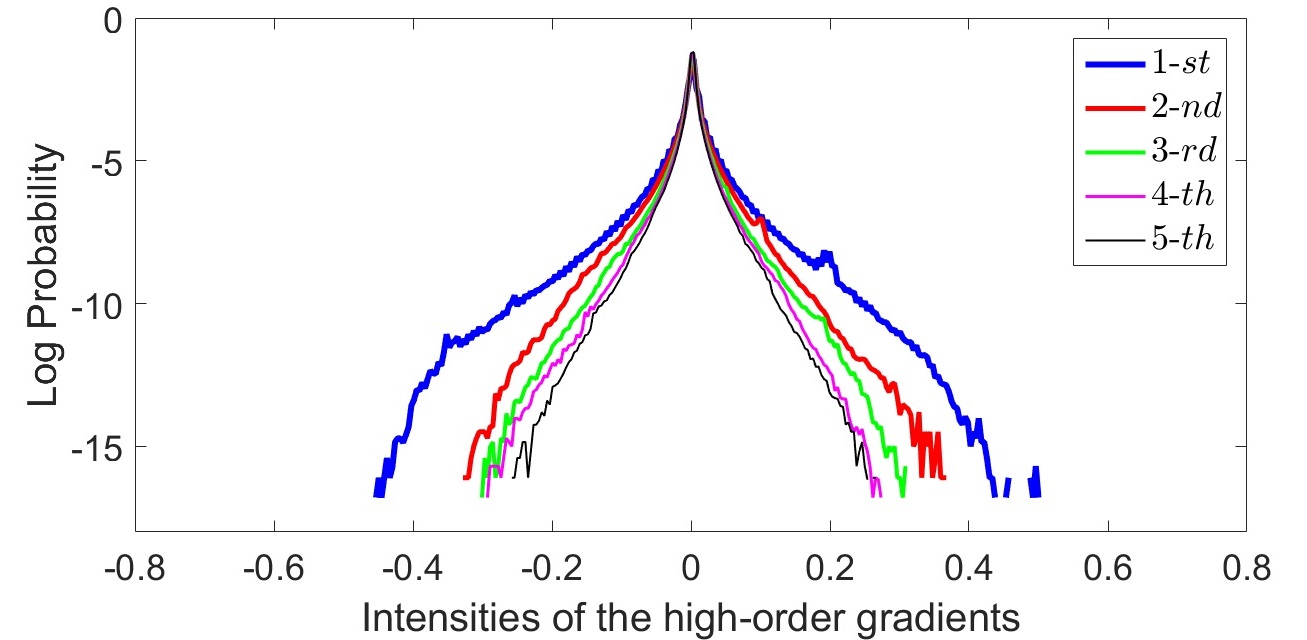
The above claims intuitively motivate us to chose $n=2$ as the highest order in most of our subsequent experiments. This choice has extra two-fold benefits: (1) $n=2$ is the simplest semi-sparsity case, and (2) the computational cost of the proposed model is also moderate when $n$ is small.

Semi-sparsity Smoothing Model

On the basis of Eq. \ref{eq:4} and verification of natural images, it is naturally to pose a semi-sparse minimization scheme for smoothing filters with the following generalized form,

\[\begin{equation} \begin{aligned} \mathop{\min}_{u} {\left\Vert {u}-{Af}\right\Vert}_2^2+\alpha \sum_{k=1}^{n-1} {\left\Vert {\nabla}^{k}u-{\nabla}^k (Af) \right\Vert}_2^p+\lambda{\left\Vert {\nabla}^{n} u \right\Vert}_0 \end{aligned} \label{eq:5} \end{equation}\]

where $\alpha$ and $\lambda$ are weights for balance. The first term in Eq. \ref{eq:5} is data fidelity with $A$ adapted from Eq. (1). The second term measures the similarity of $k$-th ($k<n$) higher-order gradients. The last term indicates that the highest-order gradient ${ {\nabla}^{n} u}$ should be fully sparse under the semi-sparsity assumptions.

In practice, the choice of $n$ is determined by the property of signals. For natural images, the observations motivate us to choose $n=2$ as the highest order for regularization. We chose $p=2$ for most filtering cases in view of the non-sparsity property of ${\nabla}^{k}u$ and low computational cost\footnote{It is possible to choose $p$ for other choices, $p=1$, for example, while the numerical solution may be computationally expensive.}. As a result, we have the reduced semi-sparsity model with the form,

\[\begin{equation} \begin{aligned} \mathop{\min}_{u} {\left\Vert {u}-{f}\right\Vert }_2^2+\alpha {\left\Vert {\nabla}u-{\nabla}f\right\Vert }_2^2+\lambda{\left\Vert \Delta u \right\Vert}_0 \end{aligned} \label{eq:6} \end{equation}\]

Here, we follow the property of global filters, letting $K$ be Kronecker kernel for simplification. This choice is based on two-fold benefits: (1) $n=2$ is the simplest case of our semi-sparsity model, and (2) a small $n$ is enough for a wide range of practical tasks with moderate computational cost.

Mathematically, Eq. \ref{eq:5} (or, \ref{eq:6}) can be viewed as a general extension of the sparsity-induced $L_0$-norm gradient regularization in the higher-order gradient cases. Despite the minor variants to $L_0$-norm gradient methods, it has startling different properties compared with many existing filtering methods. On the one hand, it has been shown in many existing filtering methods such as bilateral filter, guided filter, and TV-based filterthat it is possible to guarantee high-quality smoothing results in the polynomial-smoothing areas, but it may inevitably lead to over-smoothing effects around the sharpening edges. On the other hand, sparsity-induced models faithfully preserve the sharpening edges without over-smoothing results, but they may produce stair-case artifacts within the polynomial smoothing surfaces.

In a nutshell, it is difficult for both types of traditional filtering methods to simultaneously fit a signal coexisting the polynomial-smoothing surfaces and sparse singularities features (spikes and edges), since they may either produce over-smoothing results in singularities or introduce stair-case artifacts in the polynomial smoothing surfaces. In contrast, our semi-sparsity minimization model, as demonstrated in the following experimental parts, avoids the dilemma and it is possible to retain comparable edge-preserving properties in strong edges and spikes and more appropriate results in the polynomial-smoothing surfaces, giving arise to a so-called simultaneous-fitting ability in both spikes and polynomial-smoothing regions. This property provides a new paradigm to deal with both cases in high-level fidelity, which contributes its benefits and advantages to many traditional methods.

Half-quadratic Solver

Despite the simple form of Eq. \ref{eq:5} (or \ref{eq:6}), a direct solution is not always available due to the non-convexity and combination property of $L_0$-norm. In the literature, such a minimization problem is solved by greedy algorithms to iteratively select the sub-optimal solutions, or reduced with appropriate relaxations. Recently, different efficient algorithms such as half-quadratic (HQ) splitting, iterative hard-thresholding (IHT), and alternating direction method of multipliers (ADMM) have been proven to be suitable for $L_0$-norm regularization.

We employ the HQ splitting technique for the semi-sparsity minimization since it is easy to implement and has almost the least computational complexity for large-scale problems. The main idea of the HQ splitting algorithm is to introduce an auxiliary variable to split the original problem into sub-problems that can be solved easily and efficiently. For completeness, we briefly introduce the half-quadratic (HQ) splitting technique with a general $L_0$-norm regularized form,

\[\begin{equation} \begin{aligned} \mathop{\min}_{u} \mathcal{F}(u) + \lambda {\left\Vert Hu \right\Vert }_0 \end{aligned} \label{eq:7} \end{equation}\]

where $\mathcal{F}$ is a proper convex function, $H$ is a (differential) operator and the $L_0$-norm regularized term is a non-convex, non-smoothing but a certain separable function.

By introducing an auxiliary variable $w$, it is possible to rewrite the above minimization problem Eq. \ref{eq:7} as,

\[\begin{equation} \begin{aligned} \mathop{\min}_{u} \mathcal{F}(u) + \lambda {c(w)} + \beta {\left\Vert Hu - w \right\Vert }_2^2 \end{aligned} \label{eq:8} \end{equation}\]

where $c(w) = {\left\Vert w \right\Vert}_0$ and ${\left\Vert Hu - w \right\Vert }_2^2$ is introduced to measure the similarity of $w$ and $Hu$. The solution of Eq. \ref{eq:8} globally converges to that of Eq. \ref{eq:7} when the parameter $\beta \to \infty$.

Clearly, the proposed semi-sparsity model is a special case of Eq. \ref{eq:7}, where $\mathcal{F}(u) = {\left\Vert {u}-{f}\right\Vert }_2^2+\alpha {\left\Vert {\nabla}(u-f) \right\Vert }_2^2$ and $H$ is the Laplace operator ${\nabla}$. The optimal solution is then attainable by iteratively solving the following two sub-problems.

Sub-problem 1:

By fixing the variable $w$, the objective function of Eq. \ref{eq:6} reduces to a quadratic function with respect to $u$, giving an equivalent minimization problem,

\[\begin{equation} \begin{aligned} \mathop{\min}_{u} {\left\Vert {u}-{f}\right\Vert }_2^2+\alpha {\left\Vert {\nabla}u -{\nabla} f \right\Vert }_2^2 +\beta{\left\Vert \Delta u -w \right\Vert }_2^2. \end{aligned} \label{eq:9} \end{equation}\]

Clearly, Eq. \ref{eq:9} has a closed-form solution due to the quadratic form w.r.t. $u$. Let $\boldsymbol{D}$ and $\boldsymbol{L}$ be discrete gradient operator and Laplace operator in matrix-form, the optimal solution $u$ is then given by the following linear system:

\[\begin{equation} \begin{aligned} (\boldsymbol{I} + \alpha \boldsymbol{D}^T \boldsymbol{D} + \beta \boldsymbol{L}^T \boldsymbol{L}) u = (\boldsymbol{I} + \alpha \boldsymbol{D}^T \boldsymbol{D}) f + \beta \boldsymbol{L}^T w, \end{aligned} \label{eq:10} \end{equation}\]

where $\boldsymbol{I}$ is identity matrix. Since the left-hand side of Eq. \ref{eq:10} is symmetric and semi-positive, many solvers such as Gauss-Seidel and preconditioned conjugate gradients (PCG) methods are applicable for an efficient solution. It is also possible to use fast Fourier transforms (FFTs) for acceleration, which can significantly reduce the computational cost, in particular for a large-scale problem such as millions of variables in the context of image processing.

Sub-problem 2:

By analogy, $w$ is solved with a fixed $u$ and the first two terms in Eq. \ref{eq:6} are constant with respect to $w$, thus it is equivalent to solving the following problem,

\[\begin{equation} \begin{aligned} \mathop{\min}_{w} {\beta} {\left\Vert \Delta u -w \right\Vert }_2^2 + {\lambda}{\left\Vert w \right\Vert}_0 \end{aligned} \label{eq:11} \end{equation}\]

where $c(w)$ counts the number of non-zero elements in $w$. As demonstrated in many existing methods, Eq. \ref{eq:11} is separable and can be reduced to one-dimensional minimization problem — that is, each variable $w_i$ is estimated individually, giving by the formula,

\[\begin{equation} \begin{aligned} {w_i} = \begin{cases} 0, &\quad {\left\Vert \Delta u_i \right\Vert }_2^2<\frac{\lambda}{\beta},\\ \Delta u_i, &\quad {\left\Vert \Delta u_i \right\Vert }_2^2 \geq \frac{\lambda}{\beta}. \end{cases} \end{aligned} \label{eq:12} \end{equation}\]

It is also known that Eq. \ref{eq:12} is a hard-threshold operator and can be solved efficiently. The HQ splitting algorithm solves two sub-problems iteratively, providing an iterative scheme for the semi-sparsity minimization. Notice that both sub-problems have closed-form solutions in low computational complexity, which makes the $L_0$-norm regularized problem empirically solvable even for a large-scale of variables. The numerical results will demonstrate the effect and efficiency of the HQ splitting scheme.

The above HQ splitting scheme gives rise to an iterative hard-thresholding algorithm, the convergence of which has been extensively analyzed under convex objective function assumptions. It has shown in that such a scheme can be directly extended to non-convex $L_0$ gradient regularization for high-quality results. In , a similar iterative hard-threshold algorithm is proposed for compressed sensing, where the convergence is built under the restricted isometric property (RIP) and it is also not applicable to our case. It turns out recently that such an iterative thresholding algorithm can be extended to more general non-convex and non-smooth cases, for example, our semi-sparsity minimization, under the Kurdyka–Lojasiewicz property. The concreted discussion is out of the scope here and the interested reader is referred to the literature for more details.

Experimental Results

In this section, we show the simultaneous-fitting property of the semi-sparse minimization of Eq. \ref{eq:6} and its advantages in producing the “edge-preserving” smoothing results. We emphasize the “edge-preserving” property as it is vital for filtering tools to remove the small-scale details but preserve the sharpening variations. The proposed approach is compared with a variety of edge-aware filtering methods, including bilateral filter (BF), total variation (TV), $L_1$-TV, guided filter (GF), BM3D denoising, weighted least square (WLS) filter, $L_0$ gradient minimization , relative total variation (RTV), total generalization variation (TGV) method, and so on. The experimental results are verified on both synthetic and natural images. For the fairness of comparison, the parameters in each filtering algorithm are either configured with a greedy search strategy to give visual-friendly results or fine-tuned to reach a similar level of smoothness, qualified by the mean absolute average (MAE) or peak-signal-noise-ratio (PSNR) metrics.

Smoothing Filters:

We first simulate a $1$-D noisy signal and show the performance for persevering step-wise edges and polynomial smoothing region. As shown in Fig. (1), the cutting-edge $L_0$ gradient minimization attains high-quality results in both spikes and step-wise edges, but produces strong stair-case results in polynomial-smoothing regions. As aforementioned, the failure is largely caused by the invalidation of the sparse gradient regularization in the corresponding regions. In contrast, our semi-sparse model gives more accurate fitting results in the slope region with comparable performance in both singularities and sharpening edges.

Figure 3. An visual comparison of filtering methods over polynomial-smoothing surfaces. (a) Input, (b) BF ($w = 25$, $\delta =[8, 0.25]$), (c) GF($w=25$, $\epsilon =0.01^2$), (d) TV ($\lambda = 0.3$), (e)$L_1$-TV, (f) $L_0$ smoothing ($\lambda = 0.01, \kappa =1.05$), (g) BM3D, (h) WLS ($\alpha = 0.5$, $\lambda = 1.2$), (i) RTV ($\lambda = 0.05$, $\sigma = 2.0$), (j) TGV ($\lambda = 0.008$, $\alpha_0=0.05$, $\alpha_1 = 0.0025$), (k) Ours ($\alpha = 0.01$, $\lambda =0.02$), (l) Ground truth. PSNR: (a)-(k): 27.31, 39.10, 38.40, 39.72, 41.25, 40.50, 41.10, 41.49, 41.63, 42.52, 46.64. We compute PSNR by cropping out 12 boundary pixels for fairness comparison.

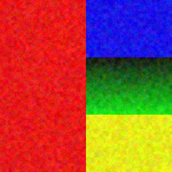
To further demonstrate the virtues of our semi-sparse smoothing filter, we compare the results of a synthesized color image that is composed of a piece of polynomial smoothing surface ({\color{green} green region}) and step-wise edges formed by different constant regions. As shown in Fig. (3), our method attains similar performance as that in the 1D case. Among them, TV method gives a high-quality fitting result within the interval of slope line, but produces over-smoothing results around the sharpening edge; $L_0$ minimization preserves the edges but leads to strong stair-case artifacts in the green region and (WLS) filter also gives a high-quality result, yet, with slight deviations in green region. The second-order TGV method significantly reduces the stair-case artifacts in the slant surface and also reveals high performance in sharpening edges, while our semi-sparsity exhibits a similar visual result and outperforms around 4 dB improvement under the PSNR metric. Other methods, to some extent, either blur the strong edges or produce piece-wise constant results in the green region.

Figure 4. Visual comparison of smoothing results on a face image. (a) Input, (b) BF ($w = 25$, $\delta =[8, 0.25]$), (c) GF ($w=25$, $\epsilon =0.01^2$), (d) TV ($\lambda = 0.2$), (e) $L_0$ smoothing ($\lambda = 0.01$, $\kappa =1.2$), (f) WLS ($\alpha = 0.5$, $\lambda = 1.2$), (g) BM3D ($\delta=30$), (h) RTV ($\lambda = 0.02$, $\sigma = 2.0$), (i) TGV ($\lambda = 0.01$, $\alpha_0=0.002$, $\alpha_1 = 0.002$), (j) Ours ($\alpha = 0.1$, $\lambda =0.02$). As suggested, the filters are processed in logarithmic intensity for better visual results. MAE: (b)-(j): 0.0115, 0.0117, 0.0118, 0.0116, 0.0117, 0.0119, 0.0117, 0.0116, 0.0117.

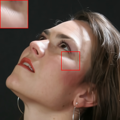
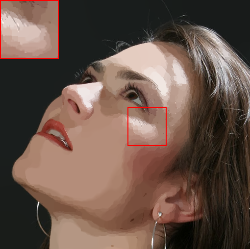
In Fig. (4), we also show the results on natural images. Specifically, we apply the filtering methods on a face image consisting of multiple polynomial surfaces (face) and strong edges (face contour and hair). In this situation, it is usually difficult to produce a visual-pleasant result. The dilemma mainly underpins the fact that both freckles and hair reveal high-frequency characteristics, while the preferred result may require to preserve the details in hair regions but to remove freckles in smoothing face regions. As shown in Fig. (4), most existing “edge-aware” filtering methods reveal limited performance in keep the smoothing balance between the high-frequency hairs and smoothing face regions. For example, bilateral filter (BF) and guided filter (GF) produce acceptable smoothing results in face regions, while they also blur the hair details slightly. BM3D method is originally proposed for image denoising and usually reveals high performance for noisy-free results, while it has limited improvement in such cases because of the complexity and diversity of potential details to be filtered out. Notice also that $L_0$ minimization produces stripe-like results in face regions. In contrast, our semi-sparsity method removes the details in face regions but also retains high-quality edges in the hair region, giving rise to a more promising results.

Figure 5. Our semi-sparsity smoothing results of an 2D image with varying parameters $\alpha$ and $\beta$. Note that the filtering algorithm is processed in the logarithmic intensity for better visual effects.

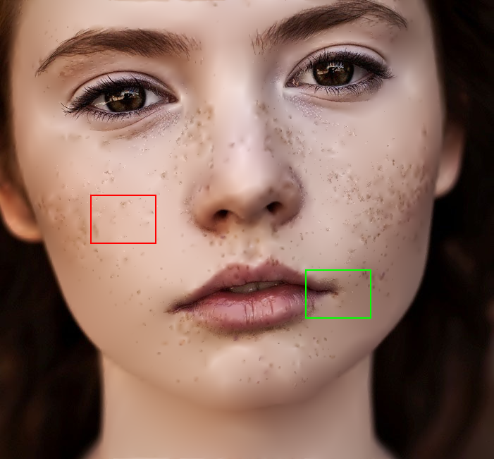
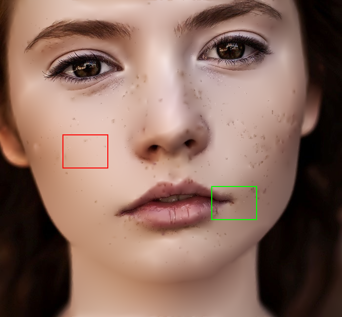
For complementary, we briefly explain the roles of ${\alpha, \beta}$ in controlling the smoothness of the semi-sparse minimization model. A visual comparison with varying parameters $\alpha$ and $\beta$ is presented in Fig. (5). In each row, $\alpha$ is fixed and $\lambda$ is gradually increased to give more smoothing results; while, in each column, $\lambda$ is fixed and $\alpha$ is increased to remove more strong local details. As we can see, $\lambda$ plays a crucial role in controlling the smoothness of results and a larger $\lambda$ penalizes to remove more local details and lead to more smoothing results. Over-weighting the second-order term will penalize smoothing regions as well as fine features and therefore over-smooth the details. A similar trend is observed for $\alpha$ but with a decreasing value and the results are not so sensitive to the varying of $\alpha$. Notice that $\alpha$ is reduced by $\kappa$ time in each iteration, because the penalty for the first-order gradient in Eq. \ref{eq:5} and \ref{eq:6} play a similar role as the data-fidelity term, thus it has a relatively small impact on the global smoothing results but mainly adjusts the local details.

Higher-order Regularization:

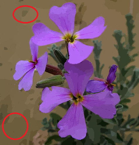
The choice of order $n$ in Eq. \ref{eq:5} for sparse regularization is generally determined by the property of signals. For natural images, we interpret that $n=2$ is usually enough to give favorable results in most cases, although further improvements can be attained with the regularization over higher-order gradient domains. As shown in Fig. (6), we illustrate this observation by comparing the smoothing results in which the sparsity constraints are imposed from the $1^{st}$ to $3^{rd}$ orders regularizations. As shown in $L_0$-gradient regularization, the $1^{st}$ order case may introduce strong staircase effects in the flower region and background. Under a similar level of smoothness, the proposed method alleviates the staircase artifacts, and no obvious difference appears except in some tiny regions for the $2^{nd}$ and $3^{rd}$ cases. This result, to some extent, provides validation of the conclusion that the regions having the degree ($n \geq 3$) polynomial surfaces in natural images occupy very tiny regions in natural images, which can be treated as spikes approximately.

Figure 6. Comparison of the smoothing results on a natural image with the sparse regularization from the $1^{st}$-order to $3^{rd}$-order gradient domains, respectively. PSNR: (b)-(d): 33.54, 33.96, 33.16 (Zoom in for better view).

This result can be also explained from the higher-order gradient distributions of natural images in Fig. 2, where the sparseness of the higher-order gradient signal is gradually enhanced when the order $n$ increases. Moreover, there exists a bound of the spareness when the order $n$ keeps increasing, as the distributions tend to be more and more similar. On the other hand, it is also clear that the gap of sparseness of the $1^{st}$ and $2^{nd}$ order gradients is much bigger than that of the $2^{nd}$ and $3^{rd}$ order gradients. A similar trend is also observed in the higher-order cases. Accordingly, we claim that the polynomial-smoothing surfaces with degree ($n \geq 3$) do not frequently occur in natural images, the area of which is relatively smaller than that of the $n=2$ case. Therefore, it is usually enough to impose sparse regularization on second-order gradients for natural images. Another consideration of choosing the $2^{nd}$ order gradient for regularization is to reduce the computation cost in many practical applications.

Applications

Similar to many existing filtering methods, it is possible to use our semi-sparsity model in various signal processing fields. We describe several representative ones involving 2D images, including image detail manipulation, high dynamic range (HDR) image compression, image stylization and abstraction.

Details Manipulation:

In many imaging systems, the captured images may suffer from degradation in details for the inappropriate focus or parameter-settings in image tone mapping, denoising, and so on. In these situations, “edge-aware” filtering methods can be used to help recover or exaggerate the degraded details. In general, it is popular to use the smoothing filters to decompose an image into two components: a piece-wise smoothing base layer and a detail layer; then either of them can be remapped and combined for reconstructing better visual results. We compare the results with the cutting-edge methods. For fairness, all filtering methods produce a similar level of smoothing results. The detail layer is then obtained by subtracting the smoothing base-layer from the original image. The enhanced image is reconstructed by combing the re-scaled ($\times 3.5$) detail layer with the base-layer. As we can see in Fig. 7, the guided filter, WLS filter, BM3D denoising and total generalization variation (TGV) methods may cause halo artifacts around strong structures; while $L_0$ smoothing helps to reduce the halos but leads to crash boundaries due to the inappropriate stair-case filtering results in the polynomial-smoothing regions. In contrast, our semi-sparsity model receives the best result with rich local details but tiny halo artifacts.

fig5_

A multi-scale strategy is also introduced for detail enhancement. As suggested in WLS filter, the multiple base layers are generated under different smoothing levels, and the detail layers are then obtained by subtracting one from the former smoothing result. As shown in Fig. (8), the small, median and coarse levels are applied for producing smoothing base layers and the final merged result.

Figure 8. Multi-scale details manipulation. Three scales: (b) small ($\alpha = 0.01, \lambda =0.001$) and (c) median ($\alpha = 0.1$, $\lambda =0.005$), (d) coarse ($\alpha = 1.0, \lambda =0.02$), and (e) is obtained by scaling ($\times 2$) detail-layers.

HDR Image Compression:

This technique arises from the visual-friendly display of high-quality HDR images. It is similar to image details manipulation and an HDR image is usually assumed to be decomposed into a base layer and a detail layer. The base layer is piece-wise smoothing with high dynamic range contrast, which needs to be compressed for display or visual purposes. The compressed smoothing output is then re-combined with the detail layer to reconstruct a new image. The challenge here is to decouple the base layer and maintain reasonable image contrast during dynamic range compression while keeping a balance of the smoothness between the piece-wise areas and sharp discontinuities to avoid halos around strong edges and over-enhancement of spatial local details.

As shown in Fig. (9), bilateral filter produces an LDR image with the fine-balance global illumination but the details in local, which is partially recovered by the gradient domain (GD) compression and WLS filter but they still have limitations in bringing out local tiny details; while $L0$ smoothing tends to produce exaggerated local details, which is mainly caused by the stair-case fitting results in polynomial smoothing surfaces. In contrast, our semi-sparse filtering method provides a result with appropriate contrast in local and fine-balanced global image illumination. A similar result is also found in Fig. (10), where we only replace the filter method and the color and saturation share the same configuration as in paper for a fair comparison. Visually, the WLS filter, guided filter, and total generalization variation (TGV) are possible to produce high-quality LDR results, but they may have limitations in compressing the dynamic range around strong edges; while our method receives a comparable result as the well-known gradient domain method. Notice that L0 smoothing method may also lead to artifacts due to the inappropriate smoothing results in the polynomial-smoothing surfaces.

Figure 9. HDR image compression. From left to right: (a) Bilateral filte (BF) (b) Gradient domain (GD) compression, (c) WLS filter, (d) $L_0$ smoothing and (e) Our result ($\alpha = 0.5, \lambda =0.01$). The results of (a)-(d) are adapted from the authors' projects. TMQI (Q): 0.8895, 0.9305, 0.8965, 0.9562.

Figure 10. HDR image compression. (a) WLS filter ($\alpha= 1.2, \lambda=5.0$), (b) Guided filter ($r=15, \delta=[8, 2]$), (c) L0 smoothing($\lambda = 0.5, \kappa = 1.2$), (d) Total generalization variation (TGV) ($\lambda = 0.02, \alpha_0=0.1, \alpha_1 = 0.05$), and (e) Ours ($\alpha = 1.0, \lambda =0.4$). For fairness, all the filters produce a similar level smoothing results under the same color and saturation configurations.TMQI (Q): 0.9681 0.9624 0.9568 0.9679, 0.9712.

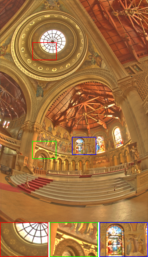
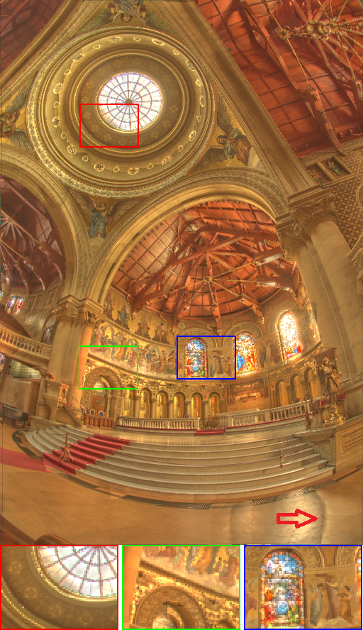
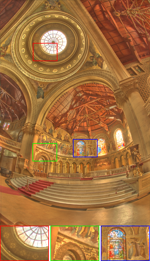
To verify the performance of these existing smoothing filters for HDR image compression, we further take a quantitative evaluation based on the Anyhere dataset. The dataset has 33 widely-used HDR images with different illumination distribution. In general, it is difficut for HDR compression tasks for an objective image quality assessment, because the corresponding ground-truth images are always not available. Recently, no-reference approaches based on statistical models have also shown promising success in predicting the quality of images. As suggested in , we use Tone Mapped Image Quality Index (TMQI), Integrated Local Natural Image Quality Evaluator (IL-NIQE) and Neural Image Assessment (NIMA) for evaluation. The TMQI index is a full-reference assessment method between HDR image and the output LDR image, in which Structural Fidelity (SF) and Statistical Naturalness (SN) are considered to provide an objective quality assessment. The SF index is based on the multi-scale structural similarity (SSIM) approach to provide a perceptual predictor of structural fidelity. The SN index is based on a statistic method to takes the natural image statistics of brightness, contrast, visibility and details into account. IL-NIQE and NIMA are two no-reference image assessments. The former is a learning method based on natural image statistics features derived from color, luminance, gradient and structure information; and the latter attempts to predict consistent aesthetic scores with human opinions using convolutional neural networks. The NIMA method is trained on a large-scale natural image dataset for perceptually-aware no-reference quality assessment. For a fairness comparison, all the filters are configured to produce a similar level smoothing results under the same color and saturation as suggested in . The statistical results are shown in \textbf{Table} \ref{tab:tab1}, where the best two results are highlighted with \textbf{bold} and \textbf{underline}, respectively. The advantages of the proposed method are also verified with consistent visual-results in Fig. (9) and (10).

Image Stylization and Abstraction:

This interesting task aims to produce different stylized results or non-photorealistic rendering (NPR) of an image. In this case, the proposed semi-sparse filtering method is firstly applied for an image to remove the local textures and details; the main structure of the smoothed image is then, as interpreted in, extracted by using the Difference-of-Gaussian (DoG) operator; and the stylized result is finally attained by merging the filter result and main structures. Due to the simultaneously-smoothing property of the semi-sparse model, it avoids introducing extra edge lines in polynomial surfaces. Despite the isotropic property of the DoG operator, it is usually enough to produce visual-friendly results. As shown in, it is also possible to produce different artistic effects such as hatching, woodcut, watercolor, and so on. We show two simple examples: pen and color-pencil drawing effects in Fig. (11). One can also combine our semi-sparse smoothing filter model with more complex configurations as illustrated in to produce more reasonable and aesthetic stylized results.

Figure 11. Image stylization. From left to right: (a) Input image, (b) Pen drawing, and (c) Color pencil effect.

Conclusion

This paper has described a simple semi-sparse minimization scheme for smoothing filters, which is formulated as a general extension of $L_0$-norm minimization in higher-order gradient domains. We demonstrate the virtue of the proposed method in preserving the singularities and fitting the polynomial-smoothing surfaces. We also show its benefits and advantages with a series of experimental results in both image processing and computer vision. One of the drawbacks is the high computational cost of solving the iterative minimization problem, which could be partially alleviated by resorting to more efficient solutions with a faster convergence rate. We leave the work for future studies.