Semi-sparsity Priors for Image Structure Analysis and Extraction
Abstract:
Image structure-texture decomposition is a long-standing and fundamental problem in both image processing and computer vision fields. In this paper, we propose a generalized semi-sparse regularization framework for image structural analysis and extraction, which allows us to decouple the underlying image structures from complicated textural backgrounds. Combining with different textural analysis models, such a regularization receives favorable properties differing from many traditional methods. We demonstrate that it is not only capable of preserving image structures without introducing notorious staircase artifacts in polynomial-smoothing surfaces but is also applicable for decomposing image textures with strong oscillatory patterns. Moreover, we also introduce an efficient numerical solution based on an alternating direction method of multipliers (ADMM) algorithm, which gives rise to a simple and maneuverable way for image structure-texture decomposition. The versatility of the proposed method is finally verified by a series of experimental results with the capability of producing comparable or superior image decomposition results against cutting-edge methods.
Introduction:
Natural images always contain various well-organized objects together with some regular/irregular textural patterns, which convey rich information for both machine and human vision. In many psychology and perception
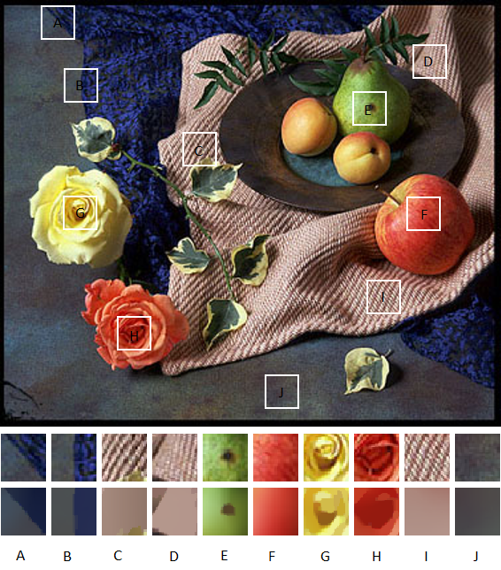
Decomposing an image into meaningful structural and textural components is generally a challenging problem due to the complex visual analysis processes. As shown in Fig. (1), visual objects could be exhibited in various and complicated forms — for example, arranged in spatial (non-)uniformly, (ir-)regularly, (an-)isotropically. The structural and textural parts, as illustrated in
In a general sense, an image is assumed to be composed of two fundamental parts: a structural part — referring to the geometrical clues, and a textural part — representing these coarse-to-fine scale details or noise
Structure and Texture Analysis
In the literature, many computational models have been developed to either extract main structures from an image or dedicate an explicit image decomposition. We review some related work regarding structural and textural analysis models for favorable image decomposition results.
Problem Formulation
We consider an additive form of the image decomposition problem — that is, given an image \(f\), it is possible to form the problem, either explicitly or implicitly, into a general optimization-based framework:
\[\begin{equation} \begin{aligned} \mathop{\min}_{u,v} \; \mathcal{S}(u)+\mathcal{T}(v), \quad \text{subject to} \quad u+v=f, \end{aligned} \label{Eq:eq1} \end{equation}\]where \(u\) and \(v\) are the structural and textural counterparts defined on \(\Omega \in \mathbf{R}^2\), typically the same rectangle or a square as that of \(f\). The functional \(\mathcal{S}(u)\) and \(\mathcal{T}(v)\) are defined in some proper spaces to characterize the properties of \(v\) and \(u\), respectively. In general, \(v\) and \(v\) could be exhibited in varying and complicated forms in natural images. In practice, \(\mathcal{S}(u)\) is advocated to capture the well-structural components such as homogeneous regions and salient edges, and \(\mathcal{T}(v)\) may be expected to have the capacity of extracting the textural part such as repeating or oscillating patterns or random noise. The generalization of \(\mathcal{S}(u)\) and \(\mathcal{T}(v)\) contributes to various existing methods in the literature.
Modeling $\mathcal{S}(u)$ for Structural Analysis
Image ``structure’’ is a vague semantic terminology and hard to give a mathematical definition. Intuitively, the structural part contributes to the majority of the semantic information of an image, which is always assumed to be composed of piece-wise constants or smoothing surfaces with discontinuous or sharpening edges. The structural analysis is devoted to finding suitable functions \(\mathcal{S}(u)\) to represent image structures. As shown in Tab. (1), \(\mathcal{S}(u)\) is typically formulated as a regularization term in the context of Eq. \ref{Eq:eq1}.
| Methods | $$ \text{Structural functional } \mathcal{S}(u)$$ | Description and References |
|---|---|---|
| Structure-aware filters | $$u = Wf$$ | Local filters |
| $$\mathcal{S}(u)= g(u, \nabla u) \|\nabla u\|^2_{2}$$ | Global filters | |
| Regularized methods | $$\mathcal{S}(u)=\alpha \|\nabla u\|_{1}$$ | TV regularization |
| $$\mathcal{S}(u)=\alpha \|\nabla u\|_{0}$$ | Gradient regularization sparsity $$ | |
| $$\mathcal{S}(u)=\alpha \|\nabla u \|_{1} +\beta \|\nabla^2 u \|_{1}$$ | $$Higher-order TV | |
| $$\mathcal{S}(u)=\alpha \|\nabla u - v \|_{1}+\beta\|\nabla v\|_{1}$$ | TGV models | |
| Patch-based Models | $$\nabla_w u:=(u(y)-u(x)) \sqrt{w(x, y)}$$ | Low-rank |
| $$\mathcal{S}(u)=\alpha\|\boldsymbol{W} \circ u\|_1+\beta\|\boldsymbol{L} \circ \boldsymbol{W} \circ u\|_1$$ | Non-local |
The early work for structure analysis can be traced back to nonlinear PDE methods for anisotropic diffusion
Another trend for image structural analysis is based on variational theory in functional spaces. For example, the pioneering Rudin–Osher–Fatemi (ROF) model
Regarding the staircase artifacts in \(\mathrm{TV}\)-based models, an effective remedy is based on higher-order methods for image structural analysis
The efforts of avoiding blurry artifacts around strong edges have also received considerable attention in image structural analysis. The sparsity-inducing \(L_0\) regularization has been demonstrated to be effective in preserving strong edges in structure-aware smoothing methods
Modeling $\mathcal{T}(v)$ for Textures or Noises
The textural part \(v\), as aforementioned, can be exhibited in diverse and complicated forms in natural images. In general, image texture is recognized as repeated patterns consisting of oscillating details, random noise, and so on. In many existing methods, the textural part \(v\) is modeled as the residual of an image \(f\) subtracting the structural part \(u\) — that is, \(v = f - u\). This simplified assumption has been adopted by many existing methods since it provides an easy but acceptable approximation for modeling image textures mathematically. The typical functional \(\mathcal{T}(v)\) for textural analysis in the literature are presented in Tab. (2). Accordingly, \(\mathcal{T}(v)\) is always treated as a data-fidelity term in the context of Eq. \ref{Eq:eq1}. We briefly discuss their advantages and limitations as follows.
| Models | Textural functional $$\mathcal{T}(v)$$ | Description and Reference |
|---|---|---|
$$f = u + v$$ |
$$\mathcal{T}(v)=\lambda \|v\|^p_p$$ | $$\|v\|^p_p= \begin{cases} \|u-f\|^2_{2}, \text{ROF model} \\ \|u-f\|_1, L^1 \text{ space} \end{cases}$$ |
| $$\mathcal{T}(v)=\lambda\|v\|_{G}$$ | $$\|v\|_{G}= \begin{cases} \inf_g \{\|g\|_{L^{\infty}} \mid v \in G\}, \\ G = \{v \mid v = \operatorname{div}g \}, \end{cases}, \text{G space} $$ | |
| $$\mathcal{T}(v)=\lambda \|v\|_{H^{-1}}$$ | $$\|v\|_{H^{-1}}=\|\nabla\left(\Delta^{-1}\right)v\|_2^2$$ | |
$$f = u + v + n$$ |
$$\lambda \|f-u-v\|_{2}^{2}+\gamma \|v\|_{G_p}$$ | $$\|v\|_{G_p}= \begin{cases} \inf \{\|g\|_{L^p} \mid v \in G_p\}, \\ G_p = \{v \mid v = \operatorname{div}g \}, \end{cases}, G_p \text{ space}$$ |
| $$\lambda \|f-K(u+v)\|_{2}^{2}+\gamma \|v\|_\ast$$ | $$\|v\|_\ast= \begin{cases} v \in W^{s,p}, \text{Sobolev space} \\ v \in H^{-s}, \text{Hilbert space}, \end{cases} $$ |
In the well-known ROF model
It has also witnessed many efforts to find more suitable functions to model the textural part \(v\) in the literature. The TV-\(G\) model
Similar to the \(G\)-norm assumption, the oscillating patterns in the Osher-Sole-Vese (OSV) model are measured in \(H^{-1}\) space given by the second-order derivative of functions in a homogeneous Sobolev space

Proposed Method
In this section, we further analyze the characteristics of image structures and textures and propose a generalized framework for image structure-texture decomposition. The model is based on a semi-sparsity-inducing regularization for structural analysis. We interpret that such a model is preferable to produce better image decomposition results in accordance with different textural analysis models.
Observations and Motivations
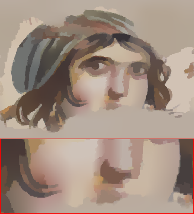
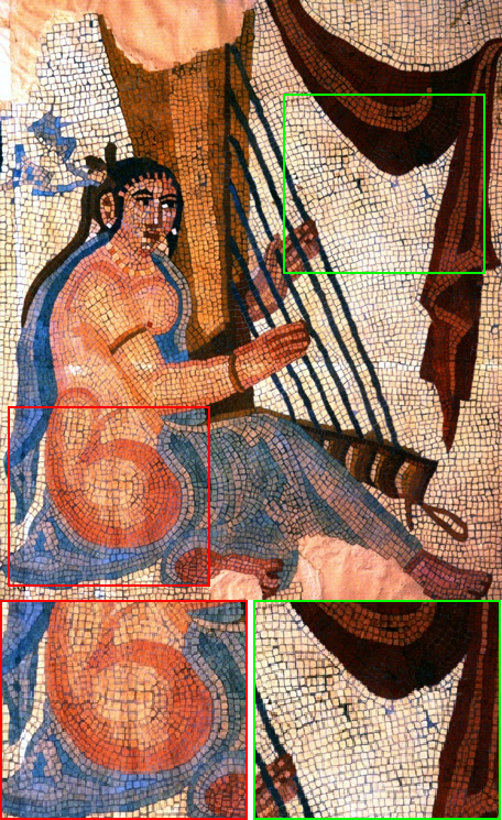
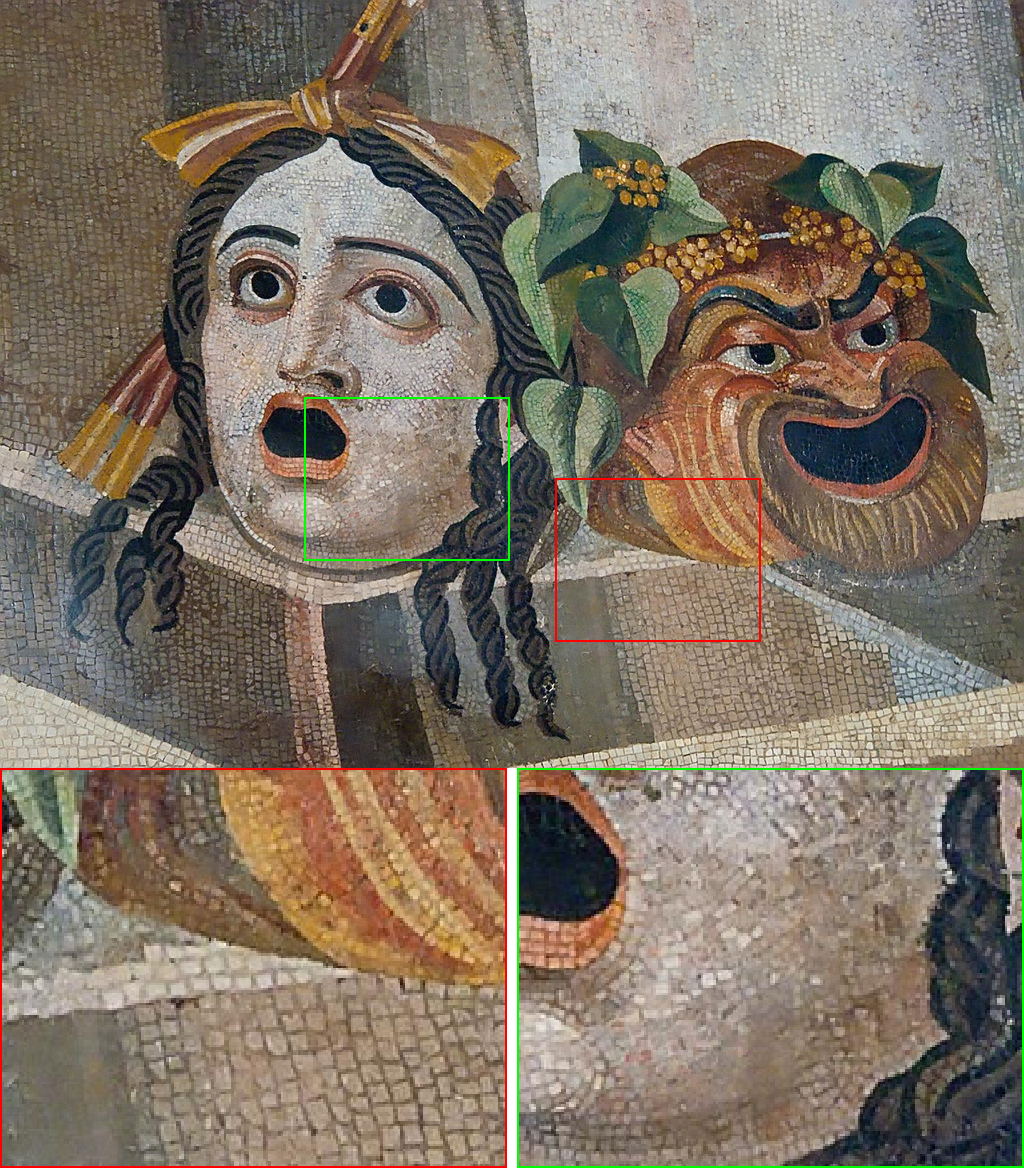
We have discussed several established image structure and texture analysis methods and highlighted their strengths and limitations for image decomposition applications. To further elucidate their properties, we first take into account an example in Fig. (2), where a natural image is given with the structural component formed by singularities, sharpening edges, polynomial-smoothed surfaces, and the textural component composed of various characteristics spanning from textural patterns, scales, and directions to amplitudes.
It is always expected for an image decomposition to ideally distinguish the structural and textural parts. But, it is a challenging problem due to the facts: (1) the sharpening edges (singularities) and oscillation patterns are highly intertwined for their high-frequent nature, but the former always belongs to image structures, and the latter is mostly attributed to image textures, (2) the piece-wise constant and polynomial smoothing surfaces may coexist in image structures, but they have very different properties and it is difficult for a simple model to capture their characteristics simultaneously, and (3) the textural part may be exhibited in various forms which are not adequate for a simple model to identify them mathematically. In summary, a plausible image decomposition method should be able to distinguish the three-fold characteristics of signals:
- Piece-wise constant or smoothing surfaces: Many natural or synthesized images have visual objects with homogeneous regions consisting of piece-wise constant and smoothing surfaces simultaneously. It is necessary for image decomposition methods to have the capacity of representing and extracting them without introducing artifacts such as staircase results in the polynomial-smoothing surfaces.
- Sharpening edges/singularities: The discontinuous boundaries between homogeneous objects give rise to sharpening edges or singularities of an image, which is important for visual understanding and analysis. An effective image decomposition model should be able to precisely preserve these features without introducing blur artifacts, and distinguish these sharpening edges and singularities from large oscillating textures\footnote{The assignment of singularities may depend on the appropriate semantic scale of the interested visual information.}.
- Coarse-to-fine oscillatory details: The characteristics of oscillatory details can be complicated because of the diverse patterns, multiple directions, varying amplitudes, and coarse-to-fine oscillation scales. It is crucial for an image decomposition method to capture these various characteristics and distinguish them from sharpening edges and singularities.
As verified in Fig. (2), the key point of image structure-texture decomposition is to distinguish the three types of signals while maintaining a fine balance. The dilemma also exists in many existing methods in Tab. (1) and Tab. (2). Structure-aware filters, for example, are capable of keeping main structures but they do not well distinguish sharpening edges and large oscillating textures. The TV-based regularization is proposed to identify the structural part with piece-wise constant and sharpening edges, while it may result in stair-case artifacts in polynomial-smoothing surfaces





(Semi)-Sparsity Inducing Regularization
“Sparsity” prior knowledge has been extensively studied in many signal and image processing fields, for example, sparse image recovering
where \(\Phi(u)\) is defined in a proper function space modeling the forward process of a physical system. The second term provides a ``sparsity’’ constraint under a linear operator \(H\) with a positive weight \(\alpha\). The notation \({\left\Vert \cdot\right\Vert }_0\) is the so-called \(L_{0}\) quasi-norm denoting the number of non-zero entries of a vector, which provides a simple and easily-grasped measurement of sparsity.
Many sparsity-inducing models can be understood in the context of Eq. \ref{Eq:eq2}. The inverse imaging reconstruction, for example, takes into account \(\Phi(u)={\left\Vert Au-f \right\Vert }_2^2\) where \(A\) is observation matrix and \(H=\nabla\) is the gradient operator because the \(L_0\) norm gradient regularization help to restore piece-wise constant image surfaces. This idea has also drawn great attention in some filtering techniques
Despite the progress in preserving discontinuous and sharp edges, the occurrence of notorious stair-case artifacts is not negligible in existing sparsity-inducing models. To address this contradiction, there has been considerable attention towards using regularization techniques in higher-order gradient domains, in particular focusing on \(\mathrm{TGV}\)-based methods
Formally, we recall the semi-sparse notations and show how to identify the semi-sparse property in the higher-order gradient domains effectively. Without loss of the generality
where \({\nabla}^{n}\) is the \(n\)-th (partial) differential operator, and \(M, N\) are some appropriate natural number satisfying \({N\gg M}\). The merit of Eq. \ref{Eq:eq3} is easy to understand, that is, the non-zeros entries of \({\nabla}^{n} u\), measured by \(L_{0}\) quasi-norm, is much smaller than that of \({\nabla}^{n-1} u\), which occurs if and only if \({\nabla}^{n} u\) is much more sparse than \({\nabla}^{n-1} u\). Taking into account a \(n\) degree piece-wise polynomial function for example, it is easy to verify that the \(n\)-th order gradient \({\nabla}^{n} u\) is sparse, while it not holds for the \(k\)-th \((k<n)\) order gradient \({\nabla}^{k} u\). It is also clear that a polynomial-smoothing signal with degree \(d<n\) satisfies Eq. \ref{Eq:eq3} essentially.


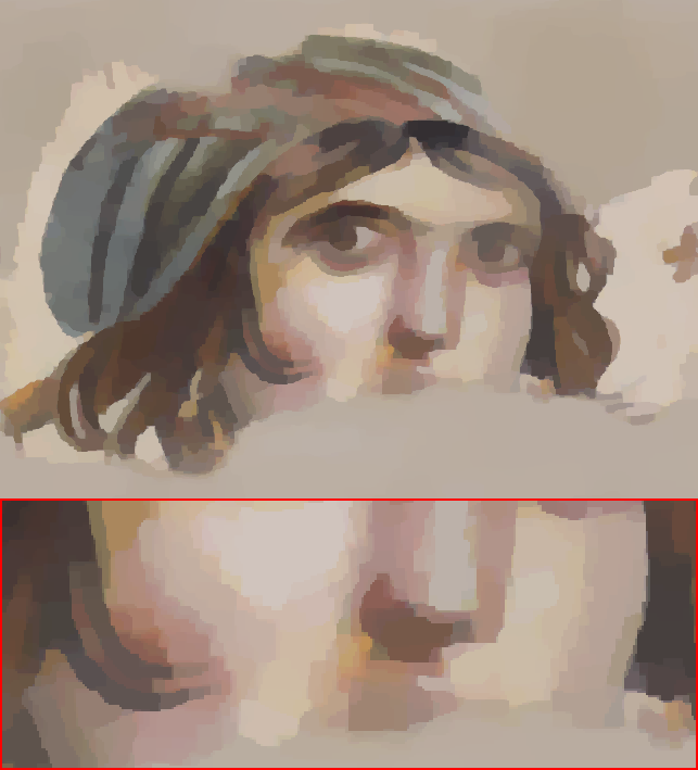
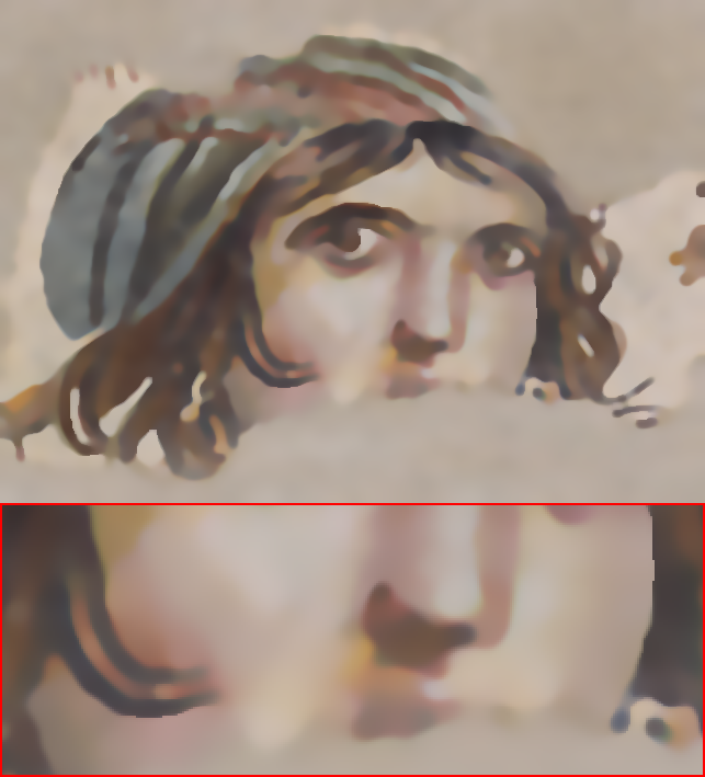

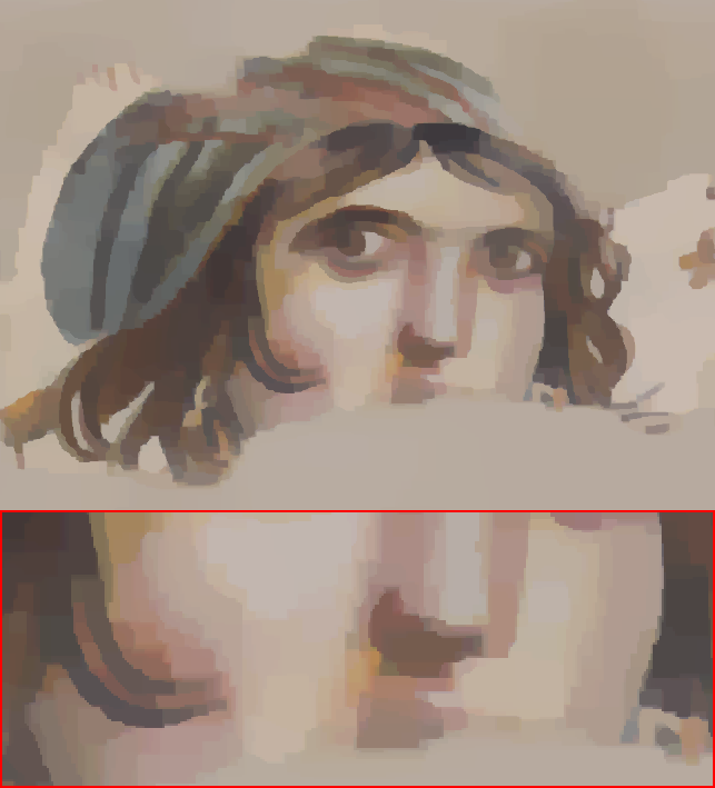
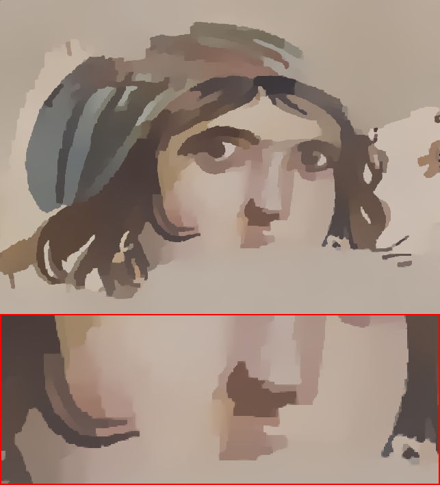
Generalized Semi-Sparse Decomposition
It has shown in the work
where \(\alpha=[\alpha_1, \alpha_2, \cdots, \alpha_n]\) are the positive weights. The semi-sparse regularization part advocates that the \(k\)-th (\(k<n\)) order gradients \({ {\nabla}^{k} u}\) have a small measure in \(L^1\) space, and the highest-order gradient \({ {\nabla}^{n} u}\) tends to be fully sparse in views of the polynomial-smoothing property of image structures. Differing from the semi-sparsity smoothing
In principle, \(\mathcal{T}(v)\) in Eq. \ref{Eq:eq4} can be arbitrarily chosen from Tab. (2). However, the textural part \(v\), as illustrated in Fig. (2), varies from image to image with diverse and multiple forms spanning from textural patterns, scales, directions to amplitudes, and so on. It is usually difficult to discriminate and describe them independently in a simple model. In this paper, we suggest using the \(L^1\)-norm to model image textures due to its simplicity and effectiveness. Firstly, it has been demonstrated in several TV-\(L^1\) models
Furthermore, the choice of \(n\) is also an important factor for the image composition model of Eq. \ref{Eq:eq4}, which is in nature determined by the property of image structures. For natural images, it has been shown in
where, \(\lambda, \alpha, \beta\) are positive parameters. Notice that \(\lambda\) is not necessarily varying in theory, for example, fixing \(\lambda=1\), and it is introduced here to rescale Eq. \ref{Eq:eq5} into an appropriate scale for a more accurate numerical solution. Despite the simple form, it enjoys some startling properties for image structure-texture decomposition. We additionally discuss the advantages and benefits of Eq. \ref{Eq:eq5} compared with many existing methods.
On the one hand, it has been shown that high-quality image decomposition results are not easy to guarantee in many existing methods, including structure-aware filters
Differing from Existing Higher-order Methods
There are two existing works highly related to the proposed semi-sparsity regularization model, in particular, the total generalization variation (TGV)
Mathematically, the TGV-based model
where \(\alpha_1, \alpha_2 \in \mathbb{R}^{+}\)are weights, and \(\xi(w)=\frac{1}{2}\left(\nabla w+\nabla w^T\right)\) denotes the distributional symmetrized derivative. Such a regularization is always combined with different textural analysis functions
The TGV-based method is essentially a second-order regularization model by introducing an auxiliary variable \(w\). Notice that \(\nabla u \approx w\) when \(\alpha_1 \to \infty\), while the exact equality is not attainable in practice, thus there exists a discrepancy between \(\nabla u\) and \(w\), in particular around sharpening edges. In this case, \(w\) can be viewed as a smoothing approximation of \(\nabla u\). Notice also that the second term \(\alpha_2 {\left\Vert \xi(w)\right\Vert}_1\) also has a smoothing role when imposing a regularization for \(w\), which may lead to over-smoothing results in sharpening edges of \(u\). The defect may be alleviated by increasing \(\alpha_1\) and reducing \(\alpha_2\), but it is not easy to find a balance in case of varying scales of oscillating textures. The intuitive conclusion is also observed in our visual comparisons. As illustrated therein, it is usually difficult to find a group of \(\alpha\) and \(\beta\) to preserve the strong edges precisely.
The \(\mathrm{TV}\text{-}\mathrm{TV}^2\) regularization is another higher-order method that has drawn attention in image restoration
The first term \(\alpha_1 {\left\Vert \nabla u\right\Vert}_1\) is a \(\mathrm{TV}\)-based regularization that encourages piece-wise constant \(u\), and the second term \(\alpha_2 {\left\Vert \nabla^2 u\right\Vert}_1\) plays a similar role but acts on the second-order gradient \(\nabla u\). The \(\mathrm{TV}\text{-}\mathrm{TV}^2\) regularization helps suppress staircase artifacts since \(\nabla u\) is imposed to be piece-wise constant. However, it is also known that the \(\mathrm{TV}\) regularization would cause blur effects around sharpening edges, and the second-order regularization would further strengthen the smoothing effect. In summary, the \(\mathrm{TV}\text{-}\mathrm{TV}^2\) regularization indeed helps reduce the stair-case artifacts but the blur results in strong edges are also not avoidable, especially in cases of large oscillating textures or strong noise. Essentially, it has a similar property as the TGV regularization.
The semi-sparsity regularization inherits the advantages of higher-order methods in terms of mitigating stair-case artifacts. In parallel, the inclusion of an \(L_0\)-norm constraint in higher-order gradients also enables the restoration of sharpening edges without compromising the fitting ability of higher-order models in polynomial smoothing surfaces. The analysis of image textures in \(L^1\) space further enhances the capacity to decompose large oscillating patterns. In summary, the proposed method combines the advantages of both TGV and \(\mathrm{TV}\text{-}\mathrm{TV}^2\), and manages to overcome their weakness, allowing image decomposition for a broad spectrum of natural images.
Efficient Multi-block ADMM Solver
The semi-sparsity image decomposition model in Eq. \ref{Eq:eq5} poses challenges in direct solution due to the non-smooth \(L^1\)-norm and non-convex nature of \(L_0\)-norm regularization. It has proved that such a minimization problem can be approximately solved based on several efficient numerical algorithms such as iterative thresholding algorithm
We here employ a multi-block ADMM algorithm to solve the proposed model because it is applicable for a type of non-convex minimization problem
where \(x_{i} \in \mathcal{X}_{i} \subset \mathbb{R}^{n_i}\) are closed convex sets, the coefficient matrix \(A_{n,i} \in \mathbb{R}^{p \times n_{i}}, b_k \in \mathbb{R}^{p}\) and \(f_{i}: \mathbb{R}^{n_{i}} \rightarrow\) \(\mathbb{R}^{p}\) are some proper functions.
The multi-block ADMM algorithm is a general case of the ADMM algorithm. Accordingly, we rewrite the Eq. \ref{Eq:eq6} in its augmented Lagrangian form,
\[\begin{equation} \begin{aligned} \mathcal{L}_{\rho} \left(\mathbf{x}, \mathbf{z}\right):=&\sum_{i=1}^{M} f_{i}\left(x_{i}\right)-\sum_{n=1}^{N}\left\langle z_n, \sum_{i=1}^{M} A_{n,i} x_{i}-b_{j}\right\rangle\\+&\sum_{n=1}^{N} \left(\frac{\rho_n}{2}\left\|\sum_{i=1}^{M} A_{n,i} x_{i}-b_{j}\right\|^{2}\right), \end{aligned} \label{Eq:eq7} \end{equation}\]where \(\mathbf{z} = \{z_1, \cdots, z_N\}\) is the Lagrange multiplier and \(\rho = \{\rho_1, \rho_2 \cdots, \rho_N; \rho_i>0\}\) is a penalty parameter. The augmented Lagrangian problem can be solved by iteratively updating the following sub-problems:
\[\begin{equation} \left\{\begin{aligned} x_{1}^{k+1} &:=\operatorname{argmin}_{x_{1}} \mathcal{L}_{\rho}\left(x_{1}, x_{2}^{k}, \cdots, x_{M}^{k} ; z^{k}\right) \\ & \quad \vdots \\ x_{M}^{k+1} &:=\operatorname{argmin}_{x_{M}} \mathcal{L}_{\rho}\left(x_{1}^{k+1}, x_{2}^{k+1}, \cdots, x_{M-1}^{k+1}, x_{M} ; z^{k}\right) \\ z_n^{k+1} &:=z_n^{k}-\rho_n \left(\sum_{n=1}^{N} A_{n,i} x_{i}^{k+1}-b_j\right)\\ \end{aligned}\right. \label{Eq:eq8} \end{equation}\]Now, it is easy to reformulate the proposed semi-sparsity image decomposition model of Eq. \ref{Eq:eq5} into a three-block ADMM model. Specifically, we consider the discrete case of Eq. \ref{Eq:eq5} and formulate it as a constrained optimization problem by introducing the variables \(\boldsymbol{h}, \boldsymbol{g}\) and \(\boldsymbol{w}\),
\[\begin{equation} \begin{aligned} \mathop{\min}_{\{\boldsymbol{u,h, g, w}\}} \; & \lambda {\left\Vert \boldsymbol{u} - \boldsymbol{f} \right\Vert }_1 + \alpha {\left\Vert \mathbf{D}\boldsymbol{u} \right\Vert }_1 +\beta {\left\Vert \mathbf{L}\boldsymbol{u}\right\Vert }_0,\\ \textit{s.t.} \quad & \; \boldsymbol{u} - \boldsymbol{f} = \boldsymbol{h}, \quad \mathbf{D}\boldsymbol{u} = \boldsymbol{g}, \quad \mathbf{L}\boldsymbol{u} = \boldsymbol{w}, \end{aligned} \label{Eq:eq9} \end{equation}\]where \(\mathbf{D}=\{\mathbf{D}_x; \mathbf{D}_y\}\) and \(\mathbf{L}=\{\mathbf{L}_{xx}; \mathbf{L}_{xy}; \mathbf{L}_{yx};\mathbf{L}_{yy} \}\) are the discrete differential operators in the first-order and second-order cases along the \(x\)- and \(y\)- directions, respectively. The augmented Lagrangian form of the three-block ADMM model of Eq. \ref{Eq:eq9} has the form,
\[\begin{equation} \begin{aligned} \mathcal{L}_{\rho} \left(\boldsymbol{u,h,g,w}; \mathbf{z}\right):= & \lambda {\left\Vert \boldsymbol{h} \right\Vert }_1+\alpha {\left\Vert \boldsymbol{g} \right\Vert }_1 +\beta {\left\Vert \boldsymbol{w}\right\Vert }_0\\ -&\left\langle \boldsymbol{z}_1, \boldsymbol{u} - \boldsymbol{f} - \boldsymbol{h} \right\rangle+\frac{\rho_1}{2} \left\|\boldsymbol{u} -\boldsymbol{f} -\boldsymbol{h}\right\|^{2}_2\\ -& \left\langle \boldsymbol{z}_2, \mathbf{D}\boldsymbol{u}-\boldsymbol{g} \right\rangle+\frac{\rho_2}{2} \left\|\mathbf{D}\boldsymbol{u}-\boldsymbol{g}\right\|^{2}_2\\ - &\left\langle \boldsymbol{z}_3, \mathbf{L}\boldsymbol{u}-\boldsymbol{w} \right\rangle+ \frac{\rho_3}{2} \left\|\mathbf{L}\boldsymbol{u}-\boldsymbol{w}\right\|^{2}_2, \end{aligned} \label{Eq:eq10} \end{equation}\]where \(\mathbf{z} = \{\boldsymbol{z}_1, \boldsymbol{z}_2, \boldsymbol{z}_3\}\) and \(\rho = \{\rho_1, \rho_2, \rho_3\}\) are the dual variables and penalty parameters adapted from Eq. \ref{Eq:eq7}. Clearly, the problem Eq. \ref{Eq:eq10} can be solved based on the iterative procedure presented in Eq. \ref{Eq:eq8}. The benefit of Eq. \ref{Eq:eq9} is that each sub-problem can be efficiently solved even for a large-scale problem. We briefly explain the sub-problems and show their property for efficient solutions.
Sub-problem $\boldsymbol{u}$ :
The augmented Lagrangian objective function Eq. \ref{Eq:eq10} reduces to a quadratic function with respect to \(\boldsymbol{u}\) when fixing the other variables, which gives rise to an equivalent minimization problem,
\[\begin{equation} \begin{aligned} \mathop{\min}_{\boldsymbol{u}} \quad &{\rho_1{\left\Vert \boldsymbol{u}-\boldsymbol{f}-\boldsymbol{h}-\frac{\boldsymbol{z}_1}{\rho_1}\right\Vert }_2^2}+{\rho_2{\left\Vert \mathbf{D}\boldsymbol{u}-\boldsymbol{g}-\frac{\boldsymbol{z}_2}{\rho_2}\right\Vert }_2^2}\\ &+{\rho_3{\left\Vert \mathbf{L}\boldsymbol{u}-\boldsymbol{w}-\frac{\boldsymbol{z}_3}{\rho_3}\right\Vert }_2^2} + c, \end{aligned} \label{Eq:eq11} \end{equation}\]where \(c\) is a constant not related to \(u\). The optimal solution of \ref{Eq:eq10} is then attained by solving the following linear system:
\[\begin{equation} \begin{aligned} (\rho_1\mathbf{I}+\rho_2 \mathbf{D}^T\mathbf{D} +\rho_3 \mathbf{L}^T\mathbf{L}) \boldsymbol{u} =& \rho_1(\boldsymbol{f}+\boldsymbol{s}) + \rho_2 \mathbf{D}^T\boldsymbol{g} +\rho_3 \mathbf{L}^T\boldsymbol{w} \\ &+ \boldsymbol{z}_1 + \mathbf{D}^T \boldsymbol{z}_2 + \mathbf{L}^T \boldsymbol{z}_3, \end{aligned} \label{Eq:eq12} \end{equation}\]where \(\mathbf{I}\), \(\mathbf{D}^T\) and \(\mathbf{L}^T\) are identity matrix and the transpose of \(\mathbf{D}\) and \(\mathbf{L}\). Due to the symmetric and positive coefficient matrix, Eq. \ref{Eq:eq12} can be directly solved using several linear solvers, for example, the Gauss-Seidel method and preconditioned conjugate gradients (PCG) method. However, these methods may be still time-consuming when the problem has a large number of variables in our cases. Notice that the differential operators \(\mathbf{D}\) and \(\mathbf{L}\) are linear invariant operators, it is possible to use fast Fourier transforms (FFTs) to solve Eq. \ref{Eq:eq12} for further acceleration. It is possible to reduce the computational cost significantly, in particular encountering a large-scale problem such as millions of variables.
Sub-problems $\boldsymbol{h}$ and $\boldsymbol{g}$:
By analogy, the sub-problems with respect to \(\boldsymbol{h}\) and \(\boldsymbol{g}\) have the forms
\[\begin{equation} \begin{aligned} \mathop{\min}_{\boldsymbol{h}} {\lambda} {\left\Vert \boldsymbol{h} \right\Vert }_1 -\left\langle \boldsymbol{z}_1, \boldsymbol{u} - \boldsymbol{f} - \boldsymbol{h} \right\rangle+\frac{\rho_1}{2} \left\|\boldsymbol{u} - \boldsymbol{f} - \boldsymbol{h}\right\|^{2}_2\\ \end{aligned} \label{Eq:eq13} \end{equation}\] \[\begin{equation} \begin{aligned} \mathop{\min}_{\boldsymbol{g}} {\alpha} {\left\Vert \boldsymbol{g} \right\Vert }_1 -\left\langle \boldsymbol{z}_2, \mathbf{D}\boldsymbol{u} - \boldsymbol{g} \right\rangle+\frac{\rho_2}{2} \left\|\mathbf{D}\boldsymbol{u} - \boldsymbol{g}\right\|^{2}_2\\ \end{aligned} \label{Eq:eq14} \end{equation}\]It is known that the optimization problem of Eq. \ref{Eq:eq13} and \ref{Eq:eq14} is a typical \(L^1\)-norm regularization minimization that can be efficiently solved for the separable property. Specifically, we reduce them into a one-dimensional minimization problem and estimate each variable \(\boldsymbol{h}_i\) and \(\boldsymbol{g}_i\) individually, giving the closed-form solutions,
\[\begin{equation} \begin{aligned} \boldsymbol{h}&=\mathcal{S}(\boldsymbol{u} - \boldsymbol{f} + \frac{\boldsymbol{z}_1}{\rho_1}, \frac{\lambda}{\rho_1}), \\ \boldsymbol{g}&=\mathcal{S}(\mathbf{D}\boldsymbol{u} + \frac{\boldsymbol{z}_2}{\rho_2}, \frac{\alpha}{\rho_2}), \end{aligned} \label{Eq:eq15} \end{equation}\]with the soft shrinkage operator defined as:
\[\mathcal{S}(x_i,\tau) = \text{sgn}(x_i)\cdot(|x_i|-\tau)_+\]where \(\text{sgn}\) is a sign function, and \((a)_+\) is defined as 0 if \(a<0\) and \(a\) otherwise.
Sub-problems $\boldsymbol{w}$:
Similarity, the sub-problem with respect to \(\boldsymbol{w}\) has the form,
\[\begin{equation} \begin{aligned} \mathop{\min}_{\boldsymbol{w}} {\beta} {\left\Vert \boldsymbol{w} \right\Vert }_0 -\left\langle \boldsymbol{z}_3, \mathbf{L}\boldsymbol{u} - \boldsymbol{w} \right\rangle+\frac{\rho_3}{2} \left\|\mathbf{L}\boldsymbol{u} - \boldsymbol{w}\right\|^{2}_2\\ \end{aligned} \label{Eq:eq16} \end{equation}\]which is a \(L_0\)-norm minimization problem and has the same separable property as \(L^1\)-norm minimization with each individual variable given by the closed-form solution
\[\begin{equation} \begin{aligned} \boldsymbol{w}=\mathcal{H}(\mathbf{L}\boldsymbol{u} + \frac{\boldsymbol{z}_3}{\rho_3}, \frac{\beta}{\rho_3}) \end{aligned} \label{Eq:eq17} \end{equation}\]where \(\mathcal{H}(x, \tau)\) is the hard-shrinkage operator defined as:
\[\begin{aligned} \mathcal{H}(x_i,\tau) = \begin{cases} 0, & |x_i| < \tau,\\ x_i, & \text{otherwise}. \end{cases} \end{aligned}\]The dual variables \(\boldsymbol{z}_1, \boldsymbol{z}_2\), and \(\boldsymbol{z}_3\) are updated as follows:
\[\begin{equation} \begin{aligned} \boldsymbol{z}_1&=\boldsymbol{z}_1 + \rho_1(\boldsymbol{u} - \boldsymbol{f} - \boldsymbol{h}), \\ \boldsymbol{z}_2&=\boldsymbol{z}_2 + \rho_2(\mathbf{D}\boldsymbol{u}-\boldsymbol{g}), \\ \boldsymbol{z}_3&=\boldsymbol{z}_3 + \rho_3(\mathbf{L}\boldsymbol{u}-\boldsymbol{w}). \end{aligned} \label{Eq:eq18} \end{equation}\]The three-block ADMM algorithm alternatively solves the sub-problems and updates the Lagrange multipliers until the given stop criteria are met, which leads to an iterative procedure for the proposed image decomposition model. Since all sub-problems have closed-form solutions in low computational complexity, the challenging non-convex \(L_0\)-norm regularized problem is empirically solvable even under a large-scale of variables. The numerical results will further demonstrate the effectiveness and efficiency of the multi-block ADMM algorithm.
The convergent analysis of multi-block ADMM solver can be directly built from the general ADMM case
Experimental Results
In this section, we further demonstrate our semi-sparse model and its high-quality decomposition performance in scenarios of images composed of different structures and textures. We start the discussion with the interpretations of a new dataset, parameter configurations, compared methods, and so on. A series of numerical results are also presented and compared with the state-of-the-art methods both qualitatively and quantitatively.
Dataset and Compared Methods
For the sake of comprehensive analysis, we first collect a new dataset for image structure and texture decomposition. This dataset has 32 images chosen from the community of image decomposition
To ensure a systematic comparison, we elaborate on our semi-sparsity model with its superior performance against a series of image decomposition methods. Specifically, we compare the model with the well-known \(\mathrm{ROF}\) model
Parameters and Configurations
Recalling the model in Eq. \ref{Eq:eq4} and \ref{Eq:eq5}, \(\lambda\), \(\alpha\), and \(\beta\) control the amount of smoothness penalty applied to output image structures. As aforementioned, \(\lambda\) is introduced to rescale Eq. \ref{Eq:eq5} into an appropriate scale, depending on the precision of discrete images and the threshold operators in Eq. \ref{Eq:eq15} and \ref{Eq:eq17}. For 8-bit color images\footnote{All images are normalized into the range \([0, 1]\) in our experiments.}, we empirically found that \(\lambda \in [0.0001, 1.0]\), \(\alpha \in [0.0001, 0.1]\) and \(\beta \in [0.0001, 0.1]\) are always suitable for a high-accuracy numerical solution when taking into account weights \(\rho_i =1 (i=1,2,3)\) without any specification. The parameters may vary from image to image depending on the density and oscillating level of image textures. The above configurations provide a good trade-off between accuracy and computational efficiency.
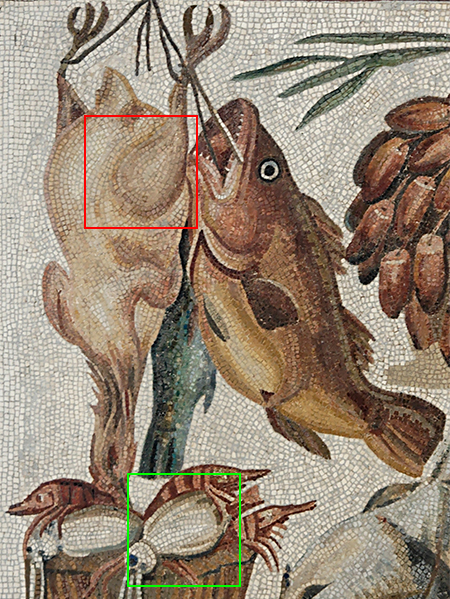
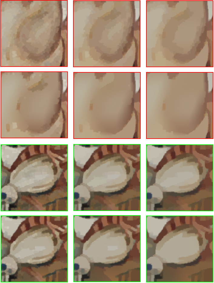
For clarity, we show the role of \({\lambda, \alpha}\) and \({\beta}\) in determining the characteristics of output image structures. As illustrated in Fig. (6), we fix \(\lambda =0.01\) and compare the output structures with varying \(\alpha\) and \(\beta\). The output image structures in each row tend to be more and more smoothing when increasing \(\alpha\), but the stair-case artifacts can not be avoided effectively in some poly-nominal smoothing regions, as \(\alpha\) mainly controls the first-order gradient to be piece-wise constant. In contrast, the staircase artifacts can be alleviated when increasing \(\beta\) in each column. This conclusion also provides the guidance for choosing \(\lambda\), \(\alpha\), and \(\beta\) in practice — that is, \(\alpha\) is first adjusted to produce acceptable decomposition results and then fine-tuning \(\beta\) to reduce the remaining stair-case artifacts to reach better local results.


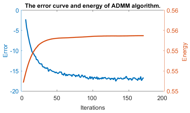
To demonstrate the efficiency of ADMM iterative procedure, we show its convergence based on the relative error \(Q_r^k ={\left\|u^{k+1}-u^k \right\|_2^2}/{\left\|u^\star\right\|_2^2}\). Notice that an ``exact’’ solution \(u^\star\) is not available here, we instead take an extremely tight stop tolerance, for example, \(\varepsilon= 10^{-16}\), and treat the output as \(u^\star\) for evaluation. Afterward, the algorithm is rerun under the same configuration with a smaller stop criterion \(\varepsilon=1.0 \times 10^{-12}\) in Algorithm 1. We also take into account the energy \(E_{u^k} = \left\|u^k\right\|_2^2\) to show the decomposition performance. The error curve \(Q_r\) and energy \(E_{u}\) are plotted in Fig. (5). As we can see, both of them converge quickly to the stable solution and it roughly needs 20 \(\sim\) 50 iterations to produce high-quality image decomposition results with appropriate parameters.
Benefiting from the multi-block ADMM procedure, the proposed model can be solved efficiently. As shown in Algorithm~\ref{Alg:alg1}, the process has three main phases: linear system solver, soft/hard-threshold shrinking operators, and the update of Lagrangian multiplier in each iteration. The computation is dominated by the linear system solver, while it can be also efficiently computed with the FFT acceleration because both the FFT and its inverse transform have the computational cost of \(O(N log(N))\), where \(N\) is the number of pixels of an image. The threshold shrinking operator can be computed independently for their separable property, and the Lagrange multiplier can be also updated in-place efficiently. As a result, the number of iterations controls the total time of the proposed method. The quantitative analysis of computational cost is also compared with the other methods in the next section.





Structure Extraction Performance
To demonstrate the benefits of the proposed method, we conduct a comparative analysis of the decomposed results. Firstly, we introduce image structure-to-texture ratio (STR) as an objective index to evaluate the smoothness of output structures, which is defined in decibels (dB) as:
\[STR = 10 \log_{10}\frac{\left\|u \right\|_2^2} {\left\|v\right\|_2^2},\]where \(u\) and \(v\) represent the decomposed image structures and textures, respectively. The STR index has the same definition as signal-to-noise (SNR) in our case when treating \(v=f-u\) as noise. For fairness, all compared methods are either configured with a greedy strategy to produce visual-friendly results or fine-tuned by hand to reach a similar smoothing level of image structures evaluated by the STR index. In what follows, we show the structural decomposition results and compare them in different scenarios of image structures and textures.
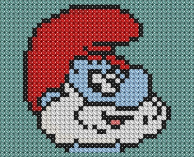
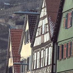

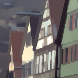
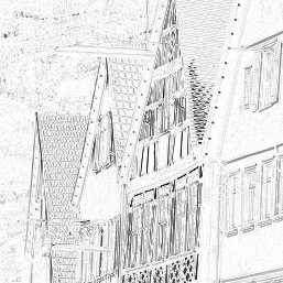
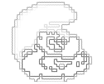
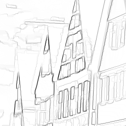
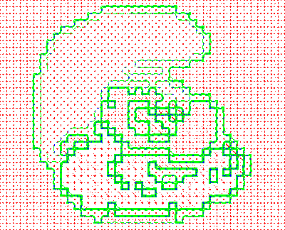
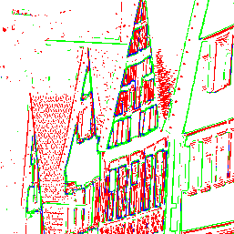
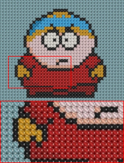
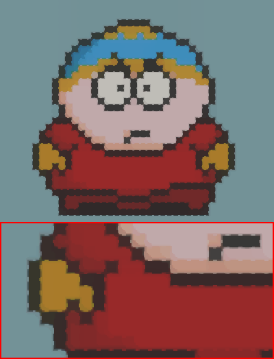
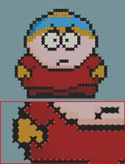
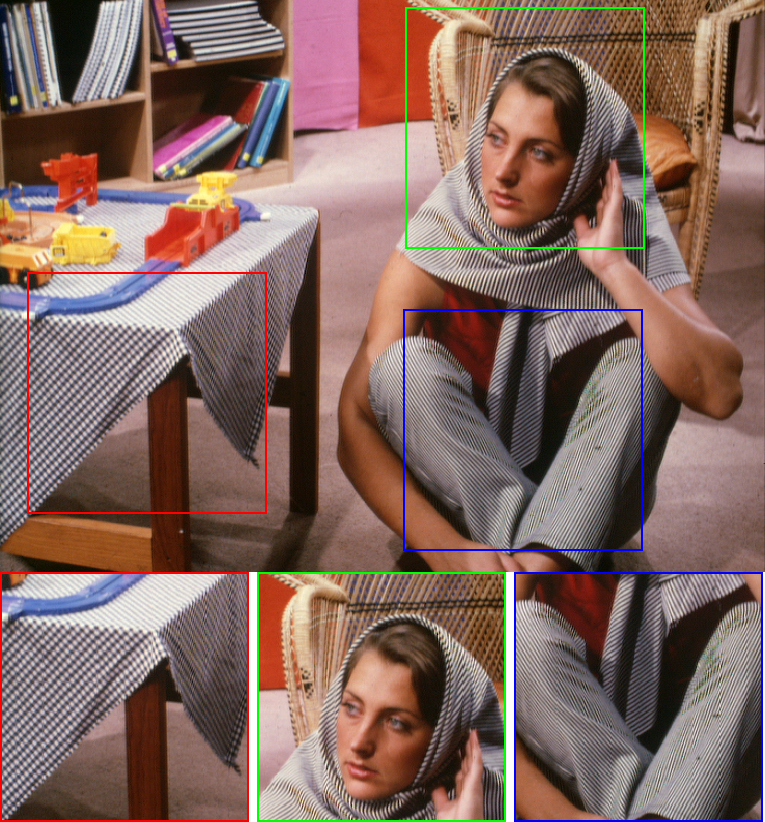
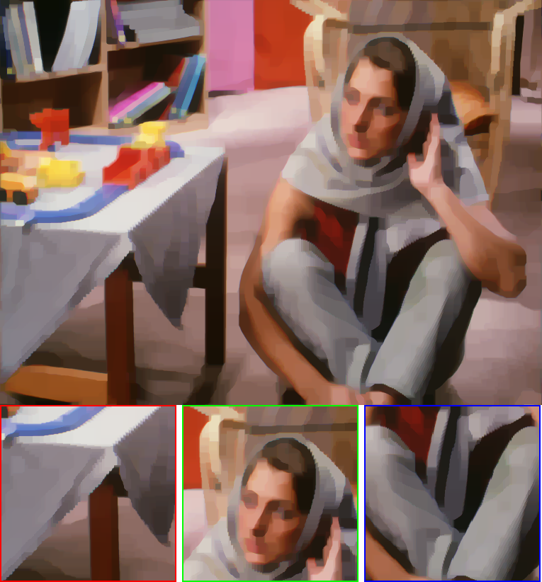
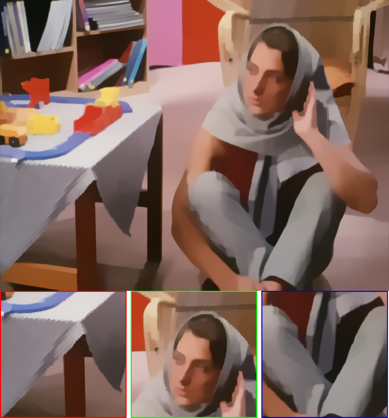
In Fig. (3), we show the decomposition structures for the first type of image. In this situation, it is usually difficult for traditional structure-aware filtering methods
We continuously analyze the second type of images by considering piece-wise constant and smoothing surfaces in structures, and multi-scale oscillating patterns in textures. As shown in Fig. (4), the TV-based ROF model
The advantage of our semi-sparsity method is further demonstrated with a more challenging case in Fig. (7). The test image here exhibits highly complex structural and textural patterns, in particular, the oscillating textures are anisotropic in directions, and have coarse-to-fine scales, and varying amplifications, which poses a significant challenge for many image decomposition models. In this case, existing methods either reveal over-smoothing results in texture-less regions or can not remove large oscillating textures, especially in view of the sharpness of discontinuous boundaries among the piece-wise constant/smoothing surfaces. Instead, the proposed semi-sparsity decomposition method gives more preferable results in this complex situation with more clean and smooth structural backgrounds and precise sharpening edges. In summary, the proposed method is applicable to a wide range of natural images and can successfully preserve sharp edges while effectively eliminating the undesired oscillating textures. The advance is mainly beneficial from the leveraging of higher-order \(L_0\) regularization for image structures and the measurement of image textures in \(L^1\) space.
Quantitative Evaluation
We further take a quantitative evaluation to compare the proposed semi-sparsity model with the aforementioned traditional methods. Notice that an objective evaluation is always not difficult for image decomposition methods because the ground truth of each component (structure or textures) is not available in practice.
| Metrics STR(19.23) | ROF | TV-L^1 | TV-G | TV-H^-1 | TV-G-𝒫 | BTF | RTV | TGV-L^1 | TGV-𝒫 | HTV-𝒫 | Ours |
|---|---|---|---|---|---|---|---|---|---|---|---|
| C_0(↓) | 0.1250 | 0.0464 | 0.0849 | 0.0462 | 0.0774 | 0.1438 | 0.0381 | 0.0850 | 0.0666 | 0.0742 | 0.0361 |
| C_1(↓) | 0.0528 | 0.0393 | 0.0400 | 0.0467 | 0.0779 | 0.1018 | 0.0442 | 0.0987 | 0.0740 | 0.1041 | 0.0239 |
| Time (s) | 5.91 | 6.31 | 11.46 | 10.82 | 16.25 | 3.61 | 2.05 | 18.20 | 22.61 | 15.52 | 12.94 |
As suggested in the work
The observation also motivates us to use the correlation coefficient for quantitative evaluation. We here define the correlation coefficient \(C(x,y)=\frac{cov(x, y)}{\sqrt{var(x) var(y)}}\) for variables \(x\) and \(y\), where \(cov(\cdot)\) and \(var(\cdot)\) refer to the covariance and variance of the counterparts, respectively. Specifically, we denote \(C_0(u,v)\) as the correlation coefficient of image structures \(u\) and textures \(v\), and \(C_1(\nabla u, v)\) as that of the gradient of image structures \(\nabla u\) and textures \(v\). Both of them are adopted to indicate the correlation between image structures and textures. For color images, each metric is computed and averaged by channel. In general, \(C_1\) is smaller than \(C_0\) due to the less correlation of the gradient \(\nabla u\) and structure \(v\). We here evaluate our semi-sparsity model against the compared methods on the new dataset. For fairness, all parameters in each method are fine-tuned by hand to give similar smoothing structures, quantified by the STR index. The correlation coefficients \(C_0\) and \(C_1\) are listed in Tab. (3), which are evaluated for each method under the average structure-to-texture ratio \(STR=19.23\) for 32 images. As we can see, the proposed semi-sparse method achieves the best results in both \(C_0\) and \(C_1\) cases.
In addition, we also compare the running time in Tab. (3) to show the efficiency of each method. To evaluate the performance of each method thoroughly, the BTF


\section {Extensions and Analysis} \label{extensions_and_analysis}
There are some obvious extensions for our semi-sparsity image decomposition model. Here, we briefly discuss two potential directions: applying the higher-order (order \(n\ge 3\)) \(L_0\) regularization for semi-sparsity priors, and replacing the textural analysis model in other spaces.
Higher-order Regularization
In the previous, we have discussed the semi-sparsity model with \(L_0\)-norm regularization in the second-order (\(n=2\)) gradient-domain in Eq. \ref{Eq:eq4} and \ref{Eq:eq5}, while it is straightforward to apply it in the higher-order (\(n\ge3\)) cases. In general, the choice \(n\) is determined by the characteristics of image signals. As illustrated in semi-sparsity smoothing filter
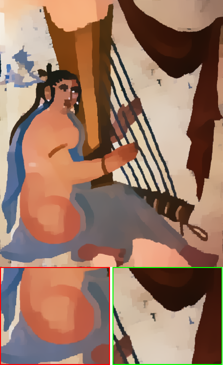
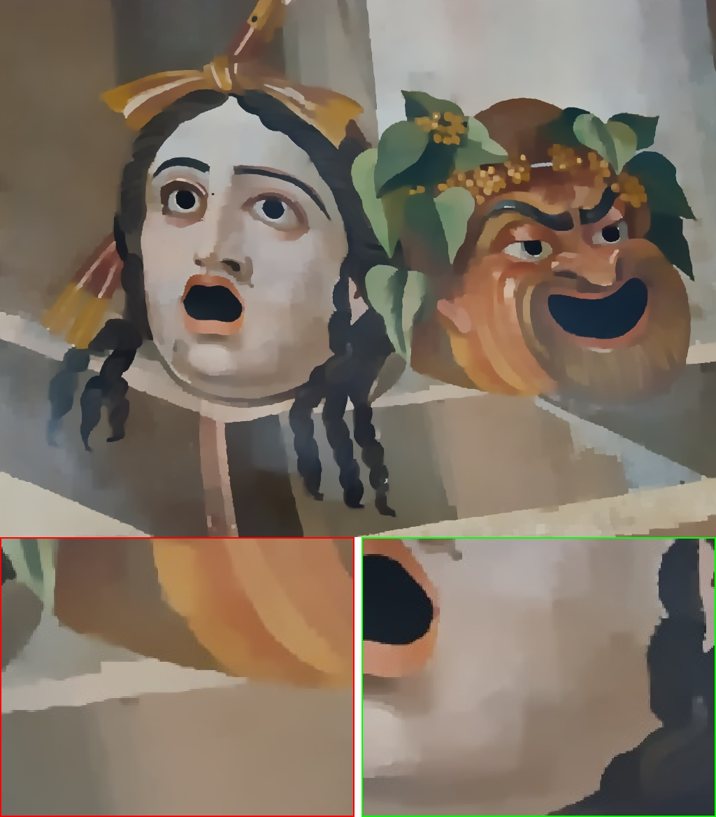

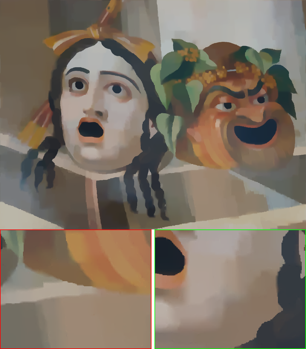
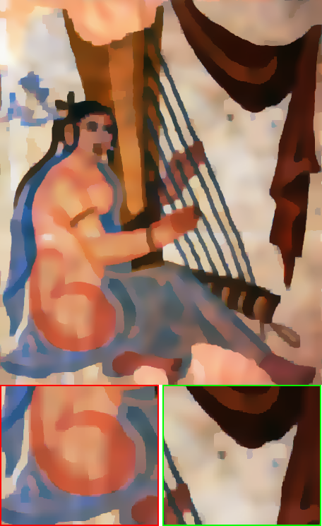
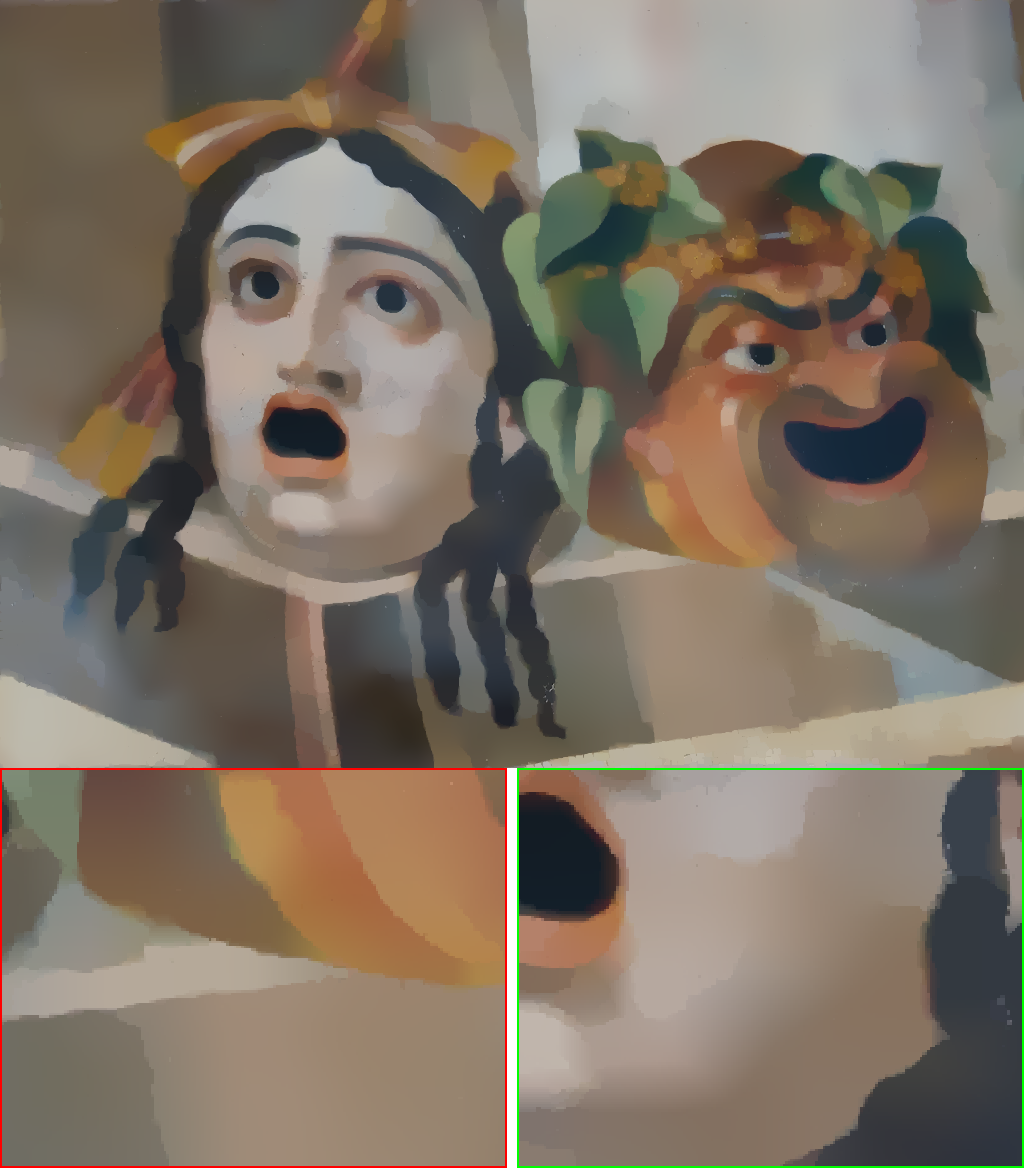
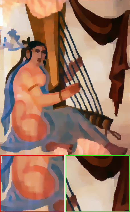

We have shown the results in different scenarios of image structures and textures by using second-order \(L_0\)-norm regularization. For complementary, we compare the results by imposing the \(L_0\) constraint on the third-order gradient domain. As shown in Fig. (9), the given image tends to have piece-wise constant and smoothing structures. In both cases, image textures are obviously removed despite that the tiny difference in the piece-wise smoothing surfaces. This is also indicated that it is usually precise enough to use second-order \(L_0\)-norm regularization. This conclusion is also demonstrated in other higher-order methods such as the well-known TGV-based methods
Textural Analysis in Different Spaces
In this paper, we have demonstrated the effectiveness of the higher-order \(L_0\)-norm regularization with the textural analysis in \(L^1\) space. Apparently, it is possible to combine such a regularization with different textural models.
As shown in Tab. (2), we have discussed several textural models that can be integrated with our structural analysis. The weak space \(G\)
where \(\operatorname{div}\) is the divergence operator. However, the direct numerical solution is unavailable for the involved \(L^{\infty}\) space. The problem is then relaxed, for example, by replacing \(G\) space with \(G_p = W^{-1,p} (1\le p<\infty)\). By analogy, we combine the semi-sparse regularization with the \(G_p\) textural analysis, giving a new semi-sparsity decomposition model,
\[\begin{equation} \begin{aligned} \mathop{\min}_{u,g} \lambda {\left\Vert u+\operatorname{div} g-f\right\Vert }_2^2+ \gamma{\left\Vert g\right\Vert }_p^p + \alpha {\left\Vert {\nabla}u\right\Vert}_1+\beta{\left\Vert \nabla^2 u \right\Vert}_0 \end{aligned} \label{Eq:eq19} \end{equation}\]where \(u = \operatorname{div} g\) with \(g\) in \(L^p\) space, and \(\lambda, \gamma\) are positive weights. The difference of Eq. \ref{Eq:eq19} from the original OSV model
Another well-known structural analysis space is based on the different specializations of Hilbert space \(\mathcal{H}\). As stated in
where \({\left\Vert f-u \right\Vert}_{H^{-1}}^2 =\int {\left\Vert \nabla\left(\Delta^{-1}\right)(f-u)\right\Vert}^2 dxdy\) for 2D cases. In the \(\mathrm{TV}-H^{-1}\) model, the oscillatory texture is modeled as the second derivative of a function in a homogeneous Sobolev space, but the underlying smooth structure may be not handled well in view of the property of \(\mathrm{TV }\) regularization, while our semi-sparsity extension in higher-order gradient domains partially avoids this problem.
For a supplement, we compare the modified models of Eq. \ref{Eq:eq19} and \ref{Eq:eq20} with the original one in \(L^1\) space. The numerical solutions are also based on the similar multi-block ADMM procedure in Algorithm 1. As shown in Fig. (10), we take two typical images into account and both of them have large oscillating textures intertwined with piece-wise constant and smoothing structures. Clearly, the textural models in weaker space \(G\) and \(H^{-1}\) tend to give similar results as the one in \(L^1\) space when combined with the semi-sparsity higher-order \(L_0\) regularization, while the one in \(H^{-1}\) space reveals slight degradation in local structural regions. An advantage of these modified models is that they tend to preserve more local structural information when compared with the cutting-edge RTV method in a similar level of smoothness. Notice also that the textural model in \(L^1\) space generally produces better visual results with more sharpening edges among the piece-wise smoothing surfaces. This may be due to the fact that the weaker space \(G\) and \(H^{-1}\) tend to capture the periodical oscillating details, while the underlying image structures and textures could be in very complicated forms. As a result, they may produce unexpected results around the irregular textural parts, for example, causing blur edges nearby the non-periodical textures. In contrast, the model in \(L^1\) space is more robust to these complex situations and this is also one of the reasons that we model the textural part in \(L^1\) space. The conclusion is also verified in Tab. (4), where the textural model in \(L^1\) space has slightly better performance in both quality and efficiency. Finally, we would like to mention that the semi-sparsity higher-order regularization can be also utilized for more complex image decomposition problems, for example, the situation of structure, texture, and noise. More exploration and discussion are out of scope here. The reader is also referred to the work
| Metrics STR(19.23) | RTV | G space | H^-1 space | L^1 space |
|---|---|---|---|---|
| C_0(↓) | 0.1444 | 0.1287 | 0.2145 | 0.0874 |
| C_1(↓) | 0.1174 | 0.0966 | 0.1383 | 0.0826 |
| Time (s) | 2.11 | 29.52 | 26.83 | 25.92 |
Conclusion
In this work, we have proposed a simple but effective semi-sparsity model for image structure and texture decomposition. We demonstrate its advantages based on a fast ADMM solver. Experimental results also show that such a semi-sparse minimization has the capacity of preserving sharp edges without introducing the notorious staircase artifacts in piece-wise smoothing regions and is also applicable for decomposing image textures with strong oscillatory patterns when applied to natural images. Some avenues of research for more complex decomposition models are also possible based on the semi-sparsity priors, which are leaving for further work.