Optimal Image Transport on Sparse Dictionaries

Abstract:
In this paper, we derive a novel optimal image transport algorithm over sparse dictionaries by taking advantage of Sparse Representation (SR) and Optimal Transport (OT). Concisely, we design a unified optimization framework in which the individual image features (color, textures, styles, etc.) are encoded using sparse representation compactly, and an optimal transport plan is then inferred between two learned dictionaries in accordance with the encoding process. This paradigm gives rise to a simple but effective way for simultaneous image representation and transformation, which is also empirically solvable because of the moderate size of sparse coding and optimal transport sub-problems. We demonstrate its versatility and many benefits to different image-to-image translation tasks, in particular image color transform and artistic style transfer, and show the plausible results for photo-realistic transferred effects.
Introduction:
Image-to-image translation is an interesting but rather challenging image synthesis problem in image processing and computer vision fields. Recent studies have shown that many vision-based tasks can be posed as a special style transfer problem within the image-to-image translation framework, for example, image color matching
In a general sense, image translation problem can be formed as an admissible map in latent feature spaces while preserving the interest of contents or information (color, texture or styles, etc.). In nature, it is necessary to solve two fundamental sub-problems, that is, image encoding and feature transformation. The former is to seek a useful image representation tool to extract the discriminative or individual image styles, while the latter aims to infer an appropriate mapping for the encoded image styles while maintaining abstract information such as image structures, textures and high-level semantic characteristics. As illustrated hereafter, many vision-based tasks can be understood from the two sub-problems. The difference mainly underpins the process of image encoding and feature transformation. Image color matching
In this paper, we propose a novel approach for image-to-image translation, in which an optimal transport map is directly posed on sparse dictionaries learned from sparse image coding. Specifically, sparse representation is applied as a feature extractor to encode the latent features of images. Optimal transport is subsequently inferred over the learned dictionaries to provide an optimal styles-swapping plan in accordance with the style encoding process. This new model, as shown in Fig. 1, inherits two-fold benefits of sparse representation and optimal transport. On the one hand, sparse representation provides us a maneuverable and easy-understood image editing tool to encode the semantic features of images, as it has been demonstrated in a variety of successful applications such as image denoising
Related work
Image-to-image translation, as aforementioned, covers a wide range of vision-based tasks despite their different backgrounds and generalizations. We briefly review some existing color transform and artistic style transfer methods, in particular the ones for photo-realistic results because of the close connections to the proposed optimal style transfer on sparse dictionaries.
Color matching or transfer is a typical image-to-image translation application keen on photo-realistic results. The purpose is straightforward, that is, to alter color appearance of an image based on a reference image
To reduce the notorious non-harmonic artifacts, recent advances based on optimal transport
Simultaneously, image style transfer — which is mostly dedicated to non-photorealistic image rendering for artistic effects, has been extensively studied for the long-standing dream of generating attractive artworks automatically. Most traditional methods are either based on line-drawing and stroke-based rendering techniques to produce the prescribed effects, including image stippling
More recently, it has also witnessed the great success of neural style transfer with the renaissance of deep learning methods. In the pioneering work
Preliminary
In this section, we briefly introduce sparse representation and optimal transport, as they form the key ingredients of the proposed model for image style (feature) encoding and transformation.
Sparse Representation:
Sparse and redundant representation
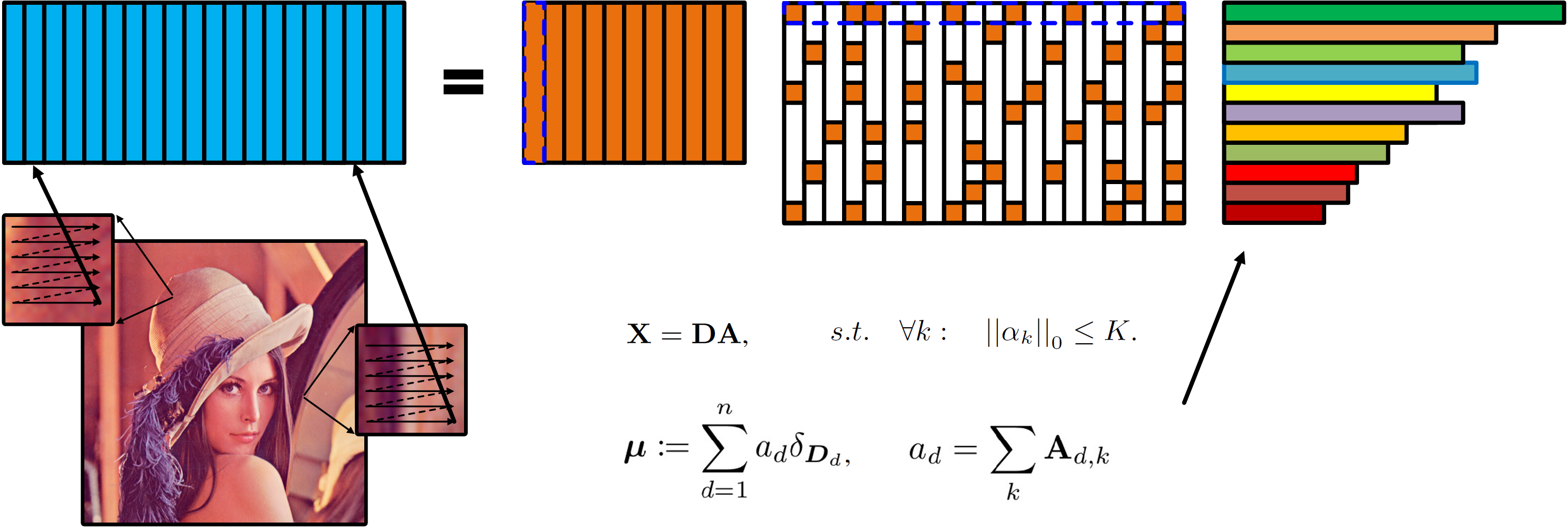
Mathematically, let \(\mathbf{X}=\{\boldsymbol{x}_i\}_{i=1}^N\),\(\boldsymbol{x}_i \in \mathbb{R}^{d}\) be a set of data samplings, for example, the vectorized image patches, sparse representation then aims to discover a group of dictionary vectors \(\{\boldsymbol{d}_j\}_{j=1}^n, \boldsymbol{d}_i \in \mathbb{R}^{d},n \ll N\) (or, denoted as \(\mathbf{D}= [\boldsymbol{d}_1, \cdots, \boldsymbol{d}_n]\)) associated with the efficient matrix \(\mathbf{A}\in \mathbb{R}^{n \times N}\), which can be written as,
\[\begin{equation} \begin{aligned} \mathbf{X} = \mathbf{D}\mathbf{A} \quad \text{s.t.} \left\|\boldsymbol{\alpha}_i\right\|_{0} \leq K, \end{aligned} \label{eq1} \end{equation}\]where \(\boldsymbol{\alpha}_i \in \mathbb{R}^{n}\) denotes the represented coefficients of sampling \(\boldsymbol{x}_i\), corresponding to the \(i\)-th column vector of the coefficient matrix \(\mathbf{A}\), \(\left\|\cdot\right\|_{0}\) is known as pseudo \(L_0\)-norm counting the non-zero elements of a vector. The constraint \(\left\|\boldsymbol{\alpha}_i\right\|_{0} \leq K\) suggests that the number of non-zero entries in \(\boldsymbol{\alpha}_i\) is no more than \(K\). In other words, the coefficient \(\mathbf{A}\) has sparse characteristics, the assumption of which forms the nature of sparse representation.
Despite the simple form, it is generally a challenging problem to give a direct solution for sparse representation because both dictionary \(\mathbf{D}\) and sparse coefficient matrix \(\mathbf{A}\) in Eq. \ref{eq1} are unknown in advance. Moreover, the solution is always not unique when solving one by fixing another. The problem is also known as an NP-hard in view of the non-convex \(L_0\)-norm constraint. In practice, it always resorts to some approximate algorithms such as the method of optimal directions (MOD)
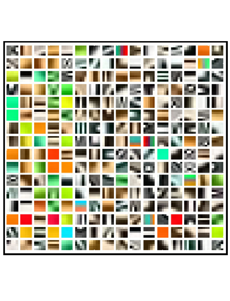
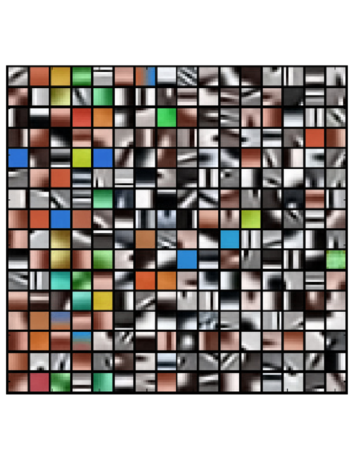
The choice of an appropriate dictionary is also crucial to sparse representation for many practical applications. We here consider an example in Fig. 2 for interpretation. The process starts with the cropped image patches that are randomly sampled from an image or a dataset. The data matrix \(\mathbf{X}\) is formed by concatenating these vectorized patches, and the dictionary \(\mathbf{D}\) and coefficient \(\mathbf{A}\) can be achieved by solving Eq. \ref{eq1} accordingly. Before diving deeper, we point here out that the row sum of the coefficient matrix is important to the proposed method, as it measures the frequency of each dictionary atom occurring in an image. Mathematically, it provides a probability distribution of image dictionary atoms. We will illustrate how to learn a pair of coupled dictionaries to represent the abstract styles of images in accordance with the optimal transport between learned dictionaries.
Optimal Transport :
Optimal transport is also a well-developed mathematical theory
The Monge’s Problem: : Let \(\mu, \nu\) be two probability measures on two metric spaces \(\mathcal{X} \in \mathbb{R}^{n},\mathcal{Y} \in \mathbb{R}^{m}\), and given a cost function \(c(x, y): \mathcal{X} \times \mathcal{Y} \rightarrow [0, \infty]\), which represents the effort of transporting the mass from \(x \in \mathcal{X}\) to \(y \in \mathcal{Y}\), the Monge’s formulation aims to find a transport map \(T: \mathcal{X} \rightarrow \mathcal{Y}\), realizing the infimum of the function:
\(\begin{equation}
\begin{aligned}
\inf_{T_{\sharp}\mu=\nu}{\int_{\mathcal{X}}{c(\mu,T(\mu)) d \nu(x)}},
\end{aligned}
\label{eq2}
\end{equation}\)
where \({T_{\sharp}\mu\stackrel{\text{def}}{=} \nu}\) is known as the \textit{push-forward} operator that pushes forward the mass of \(\mu\) to \(\nu\)
The Kantorovitch Relaxation: Alternatively, a simple relaxation of Monge’s problem initiated by Kantorovich is guaranteed to have a solution. The key idea is that the mass at any point of
\(x\) can be potentially dispatched across several locations of \(y\). The equivalent Kantorovitch formulation of the optimal transport seeks for a probabilistic coupling \(\pi \in \mathcal{P}\left(\mathcal{X} \times \mathcal{Y} \right)\) between \(\mathcal{X}\) and \(\mathcal{Y}\)
where \(\Pi\stackrel{\text{def}}{=}\left\{\pi \in\left(\mathbb{R}^{+}\right)^{\mathcal{X} \times \mathcal{Y}} \mid \pi_{\mathcal{X} }=\mu, \pi_{\mathcal{Y} }=\nu\right\}\) is the set of transportation plans with the joint distribution of marginals \(\mu\) and \(\nu\). In this formulation, \(\pi\) can be understood as a joint probability measure with marginals \(\mu\) and \(\nu\). The cost function \(c(x,y)\) can be chosen, for instance, as Euclidean distance between two locations \(x\) and \(y\), while other types of metrics could be considered, such as Riemann distances over a manifold.
Discrete Case: In practice, the distributions \(\mu\) and \(\nu\) are always accessible through discrete samples, which leads to a discrete optimal transport problem
where \(\mathbf{T}\) is a coupling matrix with entries \(\mathbf{T}_{i,j}\) describing the amount of mass flowing from \(\boldsymbol{a}_i\) to \(\boldsymbol{b}_j\) and \(\Pi(\boldsymbol{a},\boldsymbol{b}) \stackrel{\text{def}}{=} \{ \mathbf{T} \in \mathbb{R}_+^{m\times n} \vert \mathbf{T}\boldsymbol{1}_n =\boldsymbol{a}, \mathbf{T}^\top\boldsymbol{1}_m = \boldsymbol{b} \}\). The cost matrix \(\mathbf{C}\in \mathbb{R}^{m \times n}\) has the entries \(\mathbf{C}_{\boldsymbol{i,j}} = c(\boldsymbol{x}_i,\boldsymbol{y}_j)\) specifying the transport effort between the location pair \((\boldsymbol{x}_i, \boldsymbol{y}_j)\). %If \(n=m\), and \(\mu\), \(\nu\) are uniform measures, \(\Pi(\boldsymbol{a},\boldsymbol{b})\) is the Birkhoff polytope of size \(n\), and the solution of Eq. \ref{eq4} is a permutation matrix.
It is well-known that Eq. \ref{eq4} can be rewritten into a special linear program problem and solved using linear solvers such as network flow solver or transportation simplex
Optimal Image Transfer
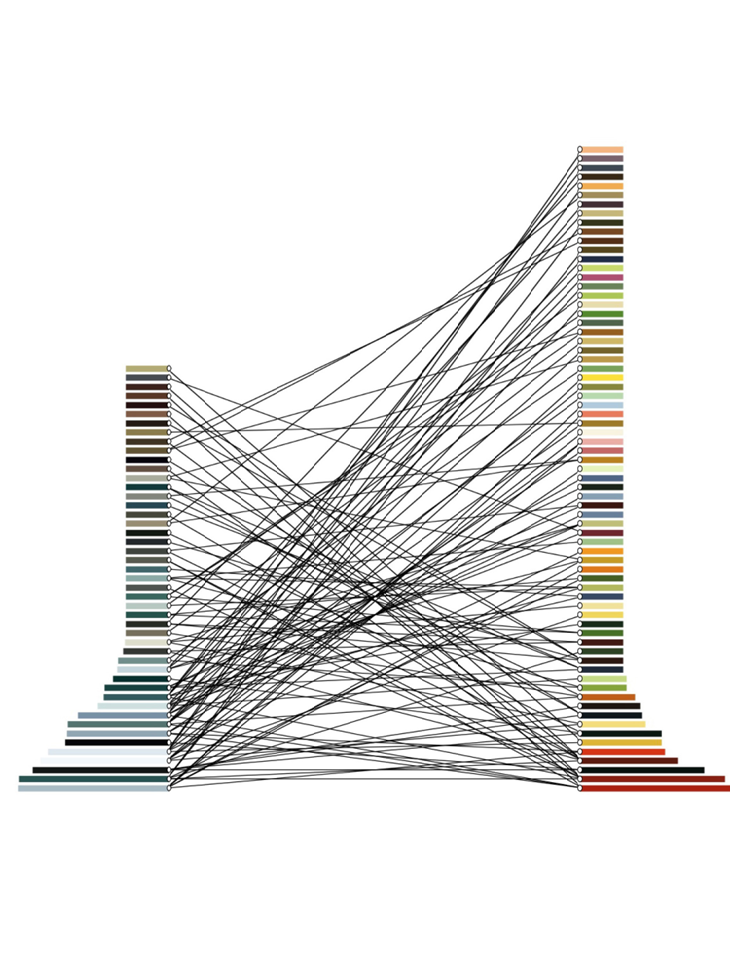
We suggest that image-to-image translation problems can be implemented by means of sparse representation and optimal transport. Image transfer, as pointed out, aims to solve the feature encoding and transformation problems. We illustrate that sparse representation provides an effective tool to encode the individual and discriminate features of different images since it has been used as a feature extractor in many image processing tasks. Sparse coefficients can be viewed as a counting process of dictionary elements, as shown in Fig. 2, which gives a probability measure to weigh the importance of each style element. Consequently, a transport plan between the encoded features is attainable and efficiently computed based on optimal transport under the small size of learned dictionaries (See Fig. 3).
Problem Formulation:
The proposed method starts with sparse representation to encode the latent styles of images and then transports the styles to reproduce a stylized image. For simplicity, we take into account an image transfer problem between two images \(x\) and \(y\) with the features or styles \(s_x\), \(s_y\), respectively. Without loss of generality, let \(\mathbf{X}=\{\boldsymbol{x}_i\}_{i=1}^M, \mathbf{Y}=\{\boldsymbol{y}_j\}_{j=1}^N, \boldsymbol{x}_i,\boldsymbol {y}_j \in \mathbb{R}^{d}\) be the vectorized patches sampled from image \(x\) and \(y\), the latent styles \(s_x\) and \(s_y\) can be expressed by sparse dictionaries given by,
\[\begin{equation} \begin{aligned} \begin{cases} &\mathbf{X} = \mathbf{D}^x\mathbf{A}, \qquad s.t. \quad {\lvert\lvert \boldsymbol{\alpha}_i \rvert\rvert}_0 \leq K_1,\\ &\mathbf{Y} = \mathbf{D}^y\mathbf{B}, \qquad s.t. \quad {\lvert\lvert \boldsymbol{\beta}_j \rvert\rvert}_0 \leq K_2, \end{cases} \end{aligned} \label{eq5} \end{equation}\]where \(\mathbf{D}^x = [\boldsymbol{d}_1^x, \cdots, \boldsymbol{d}_m^x]\) and \(\mathbf{D}^y= [\boldsymbol{d}_1^y, \cdots, \boldsymbol{d}_n^y]\) are the style dictionaries. We assume the entries \(\boldsymbol{d}_i^x,\boldsymbol{d}_j^y \in \mathbb{R}^{d}\) are in the same space. \(\mathbf{A} \in \mathbb{R}^{d\times M}, \mathbf{B} \in \mathbb{R}^{d\times N}\) contain the coefficient vectors \(\boldsymbol{\alpha}_i\) and \(\boldsymbol{\beta}_j\) of the \(i\)-th and \(j\)-th samplings \(\boldsymbol{x}_i\) and \(\boldsymbol{y}_j\). The constraints suggest the weights \(\boldsymbol{\alpha}_i\) and \(\boldsymbol{\beta}_j\) tend to be sparse — that is, the number of non-zero entries is less than the positive \(K_1\) (or, \(K_2\)).
The dictionaries \(\mathbf{D}^x\) and \(\mathbf{D}^y\), in general cases, may not exactly encode the styles \(s_x\) and \(s_y\), while, as demonstrated hereafter, it is also enough to provide favorable transferring results for image transfer tasks. The use of sparse/redundant representation, on the one hand, is to find a compact and effective image editing tool for the latent styles. Notice that the size of dictionaries is always much less than samplings in practice, thus optimal transport between two dictionaries \(\mathbf{D}^x\) and \(\mathbf{D}^y\) is affordable even using linear program solver
where \(\mathbf{C}_{i,j} \stackrel{\text{def}}{=} c(\boldsymbol{d}^x_i, \boldsymbol{d}^y_j)\) is the ground cost function to move the dictionary element \(\boldsymbol{d}^x_i\) to \(\boldsymbol{d}^y_j\), and the transport mapping function \(\mathbf{T}\) satisfies,
\[\begin{equation} \begin{aligned} \Pi(\boldsymbol{a},\boldsymbol{b}) \stackrel{\text{def}}{=} \{ \mathbf{T} \in R_+^{m\times n} \vert \mathbf{T}\boldsymbol{1}_n = \boldsymbol{a}, \mathbf{T}^\top\boldsymbol{1}_m = \boldsymbol{b}\}. \end{aligned} \label{eq7} \end{equation}\]In view of the above notations, we now interpret that the optimal style transfer over the learned style dictionaries, parameterized by \(\mathbf{T} \in R_{+}^{n \times m}\), is generalized into,
\[\begin{equation} \begin{array}{rllc} & \displaystyle \min_{\mathbf{T}} \langle \mathbf{C}, \mathbf{T} \rangle \stackrel{\text{def}}{=}\displaystyle \min_{\mathbf{T}} \sum_{i,j} \mathbf{C}_{i,j} \mathbf{T}_{i,j} & &\\ \text{s.t.} & \mathbf{D}^x\mathbf{A} =\mathbf{X}, & {\lvert\lvert \boldsymbol{\alpha}_i \rvert\rvert}_0 \leq K_1, & \\ & \mathbf{D}^y\mathbf{B} = \mathbf{Y}, & {\lvert\lvert \boldsymbol{\beta}_i \rvert\rvert}_0 \leq K_2, & \\ & \mathbf{A}\boldsymbol{1}_M=\boldsymbol{a}, & \mathbf{B}\boldsymbol{1}_N =\boldsymbol{b}, & \\ & \mathbf{T}\boldsymbol{1}_n = \boldsymbol{a}, & \mathbf{T}^\top\boldsymbol{1}_m = \boldsymbol{b}. & \end{array} \label{eq8} \end{equation}\]It is clear from Eq. \ref{eq8} that the objective function aims to infer an optimal transport plan between the learned style dictionaries, in which the first and second constraints are sparse representations for images, and the last two constraints specify the property distributions of dictionaries and the necessary conditions of transport plan. Despite the simple form of Eq. \ref{eq8}, it is not easy to solve due to the \(L_0\)-norm constraints. In what follows, a relaxed model of Eq. \ref{eq8} is further discussed with an approximate solution under some mild assumptions.
Relaxed Model: As illustrated, image style transfer is formulated into an optimal transport over sparse dictionaries with both sparse representation and optimal transport constraints. However, a direct solution to Eq. \ref{eq8} is not available due to two-fold facts: (1) the sparse coefficient constrains \({\lvert\lvert \boldsymbol{\alpha}_i\rvert\rvert}_0 \leq K_1\) and \({\lvert\lvert \boldsymbol{\beta}_i\rvert\rvert}_0 \leq K_2\) are non-convex and difficult to solve in practice; and (2) the sub-problem with respect to the variable \(\mathbf{A}\) is a typical Sylvester equation
Paying attention to \(\mathbf{A}\boldsymbol{1}_M=\boldsymbol{a}\), \(\mathbf{B}\boldsymbol{1}_N = \boldsymbol{b}\), we have \(\mathbf{X}\boldsymbol{1}_M = \mathbf{D}^x \boldsymbol{a}, \mathbf{Y}\boldsymbol{1}_N = \mathbf{D}^y \boldsymbol{b}\) by multiplying \(\mathbf{D}^x\) and \(\mathbf{D}^y\) in both sides of the third-line constraints in Eq. \ref{eq8}. As a result, a relaxed minimization problem can be written in the form,
\[\begin{equation} \begin{array}{c l l r} & \displaystyle \min_{\mathbf{T}} \langle \mathbf{C}, \mathbf{T} \rangle \stackrel{\text{def}}{=}\displaystyle \min_{\mathbf{T}} \sum_{i,j} \mathbf{C}_{i,j} \mathbf{T}_{i,j} & & \\ \text{s.t.} & \mathbf{D}^x\mathbf{A} =\mathbf{X}, & {\lvert\lvert \boldsymbol{\alpha}_i \rvert\rvert}_0 \leq K_1, & \\ & \mathbf{D}^y\mathbf{B} = \mathbf{Y}, & {\lvert\lvert \boldsymbol{\beta}_i \rvert\rvert}_0 \leq K_2, & \\ & \mathbf{D}^x\boldsymbol{a}=\mathbf{X}\boldsymbol{1}_M, & \mathbf{D}^y\boldsymbol{b}=\mathbf{Y}\boldsymbol{1}_N, & \\ & \mathbf{T}\boldsymbol{1}_n = \boldsymbol{a}, & \mathbf{T}^\top\boldsymbol{1}_m = \boldsymbol{b}. & \end{array} \label{eq9} \end{equation}\]This relaxation adores the constraints on sparse dictionaries instead of coefficients, leading to two-fold benefits. On the one hand, the constraints \(\mathbf{D}^x\boldsymbol{a}=\mathbf{X}\boldsymbol{1}_M\), and \(\mathbf{D}^y\boldsymbol{b}=\mathbf{Y}\boldsymbol{1}_N\) in Eq. \ref{eq9} change the sparse coefficient constraints into style dictionaries constraints, which helps to learn more favorable style dictionaries. On the other hand, it reduces the sub-problem with respect to \(\mathbf{A}\) (or, \(\mathbf{B}\)) into a standard sparse coding form, thereby avoiding the complex Sylvester equation. As interpreted hereafter, the relaxed problem can be approximately optimized using an alternative variable splitting method under the assumption of \(p\)-Wasserstein cost function.
The Solution of p-Wasserstein Case:
The cost function \(\mathbf{C}_{\boldsymbol{i,j}} \stackrel{\text{def}}{=} c(\boldsymbol{d}^x_i, \boldsymbol{d}^y_j)\) is important to the optimal transport plan
Recalling the relaxed model in Eq. \ref{eq9}, we first rewrite the constrained optimization problem into an unconstrained one based on regularization techniques and then apply the well-known alternative variable splitting algorithm to solve it approximately. By introducing the Lagrangian multiplier technique, the above problem can be reformulated into an unconstrained optimization problem and solved via an alternative minimization scheme as follows:
\[\begin{equation} \begin{aligned} \begin{split} \operatorname*{argmin}_{\{\mathbf{D}^x,\mathbf{D}^y, \mathbf{A},\mathbf{B}, \mathbf{T}\}} & \gamma \sum_{i,j} \mathbf{T}_{i,j} {\Vert\boldsymbol{d}^x_i-\boldsymbol{d}^y_j \Vert}^2_2 + {\big\Vert \mathbf{X}- \mathbf{D}^x \mathbf{A} \big\Vert}_{F}^2+ {\big\Vert \mathbf{Y}- \mathbf{D}^y \mathbf{B} \big\Vert}_{F}^2 \\ + & \lambda_x {\big\Vert \mathbf{X}\boldsymbol{1}_M- \mathbf{D}^x \boldsymbol{a} \big\Vert}_{F}^2 + \lambda_y {\big\Vert \mathbf{Y}\boldsymbol{1}_M- \mathbf{D}^y\boldsymbol{a} \big\Vert}_{F}^2 \\ + & \tau_x {\big\Vert\mathbf{T}\boldsymbol{1}_n - \boldsymbol{a} \big\Vert}_{2}^2 + \tau_y {\big\Vert\mathbf{T}^\top\boldsymbol{1}_m - \boldsymbol{b} \big\Vert}_{2}^2 \end{split} \end{aligned} \label{eq10} \end{equation}\]Where \(\gamma, \lambda_{x(y)}, \tau_{x(y)}\) and \(\kappa_{x(y)}\) are positive Lagrangian multipliers. Accordingly, the solution of Eq. \ref{eq10} convergent to that of Eq. \ref{eq9} when the Lagrangian multipliers go to infinity. The main idea of the alternating method is to solve the problem sequentially by fixing one variable from another. It is easy to see that Eq. \ref{eq9} can be divided into three sub-problems: sparse coding, style dictionaries learning and transport map inferring, respectively. For brevity, we describe the solution for the variables \(\mathbf{T}, \mathbf{D}^x, \mathbf{A}\), and \(\boldsymbol{a}\), and \(\mathbf{D}^y, \mathbf{B}\), and \(\boldsymbol{b}\) can be processed analogically.
Sparse coding: By fixing \(\mathbf{T}, \mathbf{D}^x, \mathbf{D}^y\) and \(\boldsymbol{a}\), \(\boldsymbol{b}\) in Eq. \ref{eq10}, the optimization problem w.r.t. the variables \(\mathbf{A}\) and \(\mathbf{B}\) is then reduced into a standard sparse encoding problem. Considering \(\mathbf{X}\boldsymbol{1}_M= \mathbf{D}^x \boldsymbol{a}\),\(\mathbf{Y}\boldsymbol{1}_N = \mathbf{D}^y \boldsymbol{b}\), the variables \(\mathbf{A}\) and \(\mathbf{B}\) only have sparse constraints. Taking the coefficient \(\mathbf{A}\) for example, the representation vectors \(\boldsymbol{\alpha}_i\) for each example \(\boldsymbol{x}_i\) in \(\mathbf{X}\) is the \(i\)-th column of \(\mathbf{A}\), which is attained by solving the following problem,
\[\begin{equation} \begin{aligned} \min_{\boldsymbol{\alpha}_i} {\lvert\lvert \boldsymbol{\alpha}_i \rvert\rvert}_0, \quad s.t. \quad \boldsymbol{x}_i = \mathbf{D}^x\boldsymbol{\alpha}_i. \end{aligned} \label{eq11} \end{equation}\]As aforementioned, the sparse coding problem of Eq. \ref{eq11} can be solved by many existing methods such as matching pursuit (MP) or orthogonal matching pursuit (OMP) algorithms
Learning style dictionaries: By analogy, we then fix the coefficients \(\mathbf{A}, \mathbf{B}\) and transport map \(\mathbf{T}\) and update the style dictionaries \(\mathbf{D}^x\) and \(\mathbf{D}^y\), respectively. Considering the relaxed constraints \(\mathbf{X}\boldsymbol{1}_M= \mathbf{D}^x \boldsymbol{a}, \mathbf{Y}\boldsymbol{1}_N = \mathbf{D}^y \boldsymbol{b}\), we rewrite the Tikhonov regularization form of the sub-problem of Eq. \ref{eq10} with respect to \(\mathbf{D}^x\) (or, \(\mathbf{D}^y\)) as,
\[\begin{equation} \begin{aligned} \begin{split} \operatorname*{argmin}_{\{\boldsymbol{d}^x_i\}} &{\Vert \mathbf{D}^x\mathbf{A} - \mathbf{X} \Vert}_{F}^2 + \lambda_x {\Vert \mathbf{D}^x \boldsymbol{a} - \mathbf{X}\boldsymbol{1}_M \Vert}_{2}^2 \\+& \gamma \sum_{i,j} \mathbf{T}_{i,j} {\Vert\boldsymbol{d}^x_i-\boldsymbol{d}^y_j \Vert}^2_2 \end{split} \end{aligned} \label{eq12} \end{equation}\]where \(\lambda_x\) and \(\tau_x\) are the positive weights. Accordingly, Eq. \ref{eq10} can be viewed as a regularized dictionary learning problem. To learn the redundant style dictionaries, we use the famous K-SVD algorithm
The Extended K-SVD Algorithm: In the K-SVD algorithm
where \(\mathbf{E}^k=\mathbf{X}- \sum_{j \neq k} \boldsymbol{d}^x_j \boldsymbol{\alpha}_{T}^j\) is the residual part that not involves the \(k\)-th dictionary element \(\boldsymbol{d}^x_k\), and \(\alpha_{T}^k\) is the \(k\)-th row of the coefficient matrix \(\mathbf{A}\). With the above form, \(\boldsymbol{d}_i^x\) is updated as the first left eigenvector given by SVD algorithm based on the K-SVD algorithm
The process can be analogically extended to the regularization case. Let \(\mathbf{E}^k =\mathbf{X}-\sum_{k\neq i} \boldsymbol{d}_k^x \boldsymbol{\alpha}_{k}^T\) and \(\mathbf{F}^k= \mathbf{X}\mathbf{1}_{M}-\sum_{k\neq i} \boldsymbol{d}_k^x \boldsymbol{a}_{k}^T\) be the residual of \({\Vert \mathbf{D}^x\mathbf{A} - \mathbf{X} \Vert}_{F}^2\) and \({\Vert \mathbf{D}^x \boldsymbol{a} - \mathbf{X}\boldsymbol{1}_M \Vert}_{2}^2\) without using the element \(\boldsymbol{d}_i^x\), where \(\boldsymbol{\alpha}_{k}\) and \(\boldsymbol{a}_{k}\) are the \(k\)-th row vector of \(\mathbf{A}\) and \(\boldsymbol{a}\). With this notation, the first two terms in Eq. \ref{eq12} can be rewritten as \({\Vert \mathbf{E}^k -\boldsymbol{d}_i^x \boldsymbol{\alpha}_{i}^T \Vert}_{F}^2\) and \({\Vert \mathbf{F}^k - \boldsymbol{d}_i^x \boldsymbol{a}_{i}^T \Vert}_{F}^2\), respectively. The sub-problem Eq. \ref{eq12} with respect to the \(k\)-th dictionary \(\boldsymbol{d}^x_k\) can be rewritten into the form,
\[\begin{equation} \begin{aligned} \begin{split} \operatorname*{argmin}_{\boldsymbol{d}^x_k} & \left\| \mathbf{E}^k- \boldsymbol{d}^x_k \boldsymbol{\alpha}_{T}^k \right\|_{F}^2 + \lambda_x \left\| \mathbf{F}^k- \boldsymbol{d}^x_k \boldsymbol{a}_{T}^k \right\|_{F}^2 + & \gamma \sum_{j} \mathbf{T}_{k,j} {\Vert\boldsymbol{d}^x_k-\boldsymbol{d}^y_j \Vert}^2_2. \end{split} \end{aligned} \label{eq14} \end{equation}\]It is easy to verify that \(\boldsymbol{d}_i^x\) has a closed-form solution because the objective function in Eq. \ref{eq14} is quadratic with respect to \(\boldsymbol{d}^x_k\). The last two terms in Eq. \ref{eq14} can be treated as the regularization terms compared with Eq. \ref{eq13} and such a regularization also helps to strengthen a more stable numerical solution. The reader is referred to the K-SVD algorithm
Optimal Transport: The transport mapping \(\mathbf{T}\) over the learned style dictionaries is a standard optimal transport problem when fixing the style dictionaries \(\mathbf{D}^x, \mathbf{D}^y\) and coefficients \(\mathbf{A}, \mathbf{B}\), that is,
\[\begin{equation} \begin{aligned} \begin{split} &\operatorname*{argmin}_{\mathbf{T}} \ \sum_{i,j} \mathbf{T}_{i,j} {\Vert\boldsymbol{d}^x_i-\boldsymbol{d}^y_j \Vert}^2_2, \\ & s.t. \quad \mathbf{T}\boldsymbol{1}_n = \boldsymbol{a}, \ \mathbf{T}^\top\boldsymbol{1}_m = \boldsymbol{b}. \end{split} \end{aligned} \label{eq15} \end{equation}\]It is worth noting that a discrete optimal transport can be solved by linear programming, while the computational cost increases significantly over the large-scale samplings
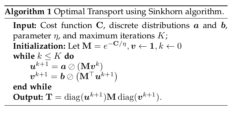
Entropy-Regularized Optimal Transport: It is well-known that an exact solution to optimal transport based on the network flow method has computational complexity \(O\left(n^3\right)\) for the \(n\) samplings
where \(H(\mathbf{T}) = \sum_{i,j}\mathbf{T}_{i,j} (log (\mathbf{T}_{i,j})-1)\) is the negative entropic regularization, and \(\eta\) is the positive regularization parameter. As interpreted in
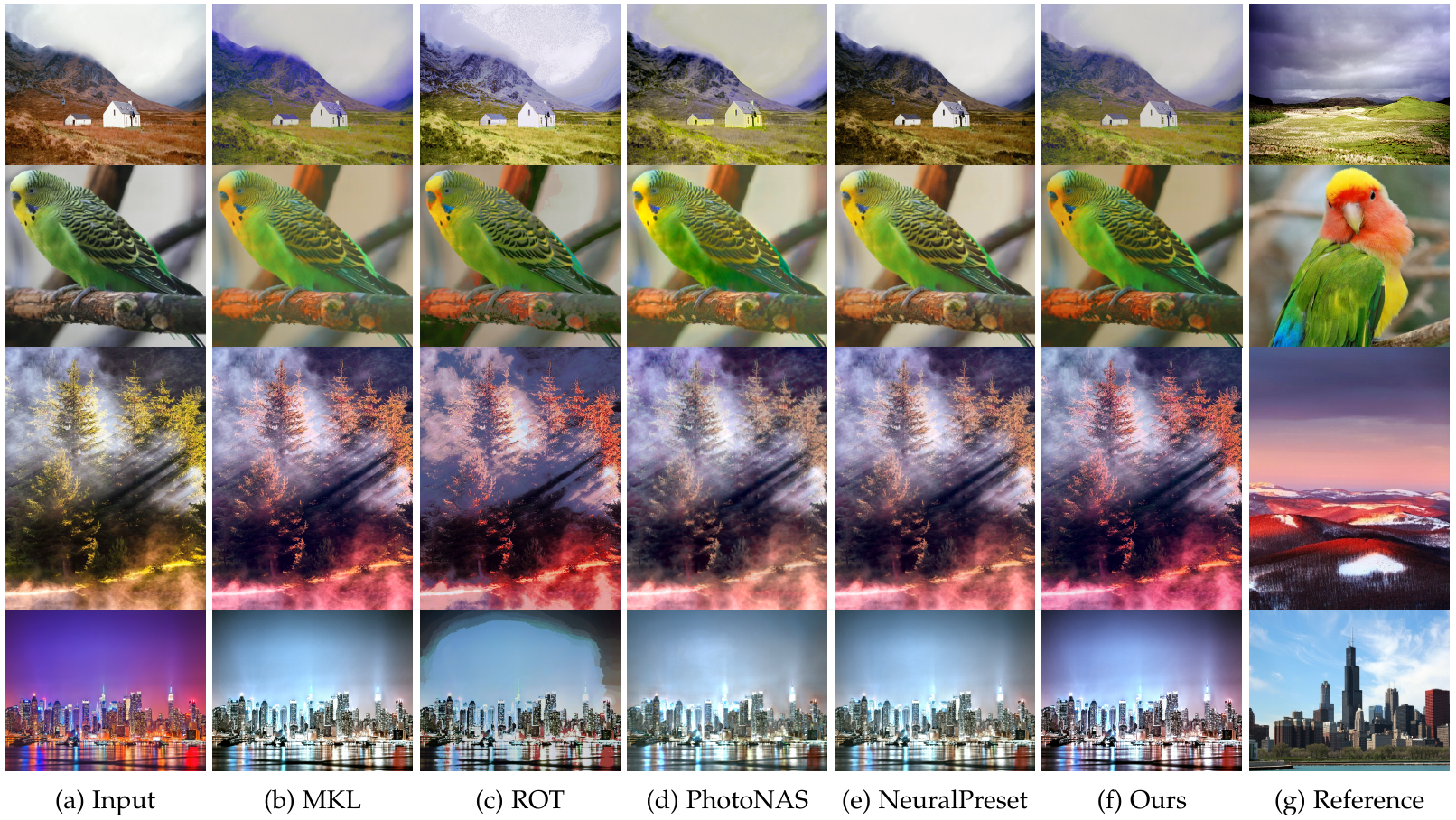
Image Synthesis:
Once the dictionaries \(\mathbf{D}^{x}\) and \(\mathbf{D}^{y}\) and transport map \(\mathbf{T}\) are obtained, given an image \(\mathbf{x}\) in style \(s_{x}\), it is then easy to reconstruct an image \(\hat{\mathbf{y}}\) with the style \(s_{y}\) by swapping the corresponding style dictionaries but keeping the sparse representing coefficients invariant, that is,
\[\begin{equation} \begin{split} \hat{\mathbf{y}}_i= \hat{\mathbf{D}}^{x} \boldsymbol{\alpha}_i =\mathbf{T}({\mathbf{D}}^{y}) \boldsymbol{\alpha}_i, \end{split} \label{eq17} \end{equation}\]where the \(k\)-th column of \(\hat{\mathbf{D}}^{x}\) is \(\hat{\boldsymbol{d}}^{x}_i=\mathbf{T}(\boldsymbol{d}^{y}_j)=\frac{\sum_{j=1}^n \mathbf{T}_{i,j} \boldsymbol{d}^y_j}{\sum_{j=1}^n \mathbf{T}_{i,j}}\), which can be viewed as a posterior mean estimate to define a one-to-one of the transfer function
where \(\nabla\) is the gradient operator and \(\rho\) is the parameter to weight the gradient regularization term. It is easy to verify that Eq. \ref{eq18} can be easily computed due to its closed-form solution.
Experiment Results
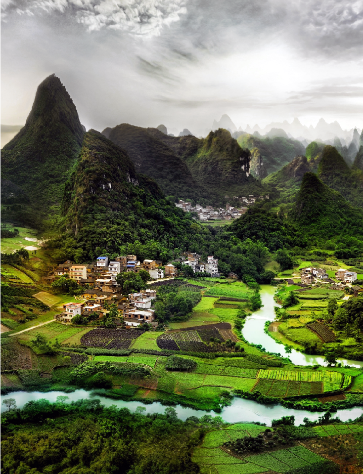
In this section, we extensively illustrate the performance of optimal style transfer and show the empirical evidence on two fundamental image-to-image translation tasks: color transform and artistic style transfer. In each scenario, the sparse coefficients and individual dictionaries are firstly learned using sparse representation and then an optimal transport map is derived on the learned dictionaries (See Fig. Fig. 1). The process is updated iteratively until it converges to a given stop criteria. The learned dictionaries are treated as individual feature styles for image reconstruction.
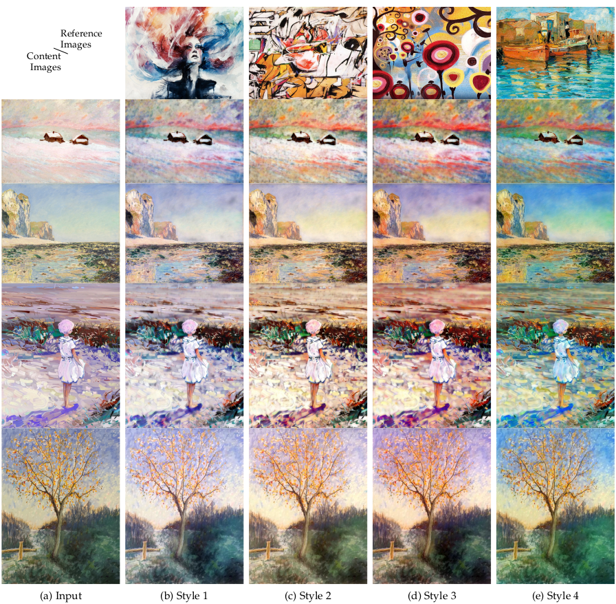
As shown in Fig. 6, the OT-based MKL mapping
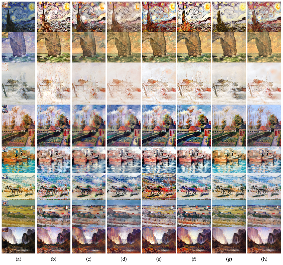
Photo-realistic Style Transfer:
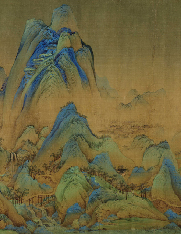
We further show that the proposed model is applicable to artistic style transfer, especially the photo-realistic effects. As shown in Fig. 6, we present the transferred results with the artworks created by famous artists. It is clear that all cases have very complex content information composed of sophisticated painting strokes and multiple colors, and textures for aesthetic effects. To receive visual-pleasant results, we randomly select \(100K\) patches from content and reference images, and use \(1024\) dictionary elements for training. The optimal transport is solved by the entropy-regularized method
In Fig. Fig. 8, we compare the transferred results with deep learning-based methods. The AdaIN model
Additionally, we present the quantitative performance against recent deep learning-based methods. Notice that an objective assessment is often difficult due to the lack of ground truth in aesthetic significance. As suggested in recent work
The evaluation is conducted on a small subset with 21 paired content and reference images sampled from of the WikiArt dataset