Intrinsic Image Transfer for Illumination Manipulation

Figure 1. Image illumination and reflectance mapping in the logarithmic intentsity domain. From (a)-(d) top: local illumination mapping (a=[0.3, 0.1, -0.1, -0.3]), middle: global illumination mapping (b=[0.6, 0.9, 1.1, 1.4]), bottom: global reflectance mapping (c=[0.5, 0.8, 1.2, 1.5]).

Abstract:

We present a novel intrinsic image transfer (IIT) algorithm for image illumination manipulation, which creates a local image translation between two illumination surfaces. This model is built on an optimization-based framework composed of illumination, reflectance and content photo-realistic losses, respectively. Each loss is firstly defined on the corresponding sub-layers factorized by an intrinsic image decomposition and then reduced under the well-known spatial-varying illumination illumination-invariant reflectance prior knowledge. We illustrate that all losses, with the aid of an “exemplar” image, can be directly defined on images without the necessity of taking an intrinsic image decomposition, thereby giving a closed-form solution to image illumination manipulation. We also demonstrate its versatility and benefits to several illumination-related tasks: illumination compensation, image enhancement and tone mapping, and high dynamic range (HDR) image compression, and show their high-quality results on natural image datasets.

Intrinsic Images Model

In many existing Retinex-based model , an image $\mathcal{I}$ is assumed to be factorized into illumination $\mathcal{L}$ and reflectance $\mathcal{R}$,

\[\begin{equation}\label{eq:eq1} \begin{aligned} \mathcal{I=L\odot R,} \end{aligned} \end{equation}\]

where ${\odot}$ is a point-wise multiplication operator, $\mathcal{L}$ represents the light-dependent properties such as shading, shadows or specular highlights of images, and $\mathcal{R}$ represents the material-dependent properties, known as the reflectance of a scene. $\mathcal{L}$ and $\mathcal{R}$ take rather different roles in controlling the image color, contrast, brightness and so on. Such an image decomposition has formed a basis for many intrinsic image decomposition methods.

Limitations: Eq. (\ref{eq:eq1})is a highly under-constraint problem if no further assumption is imposed on illumination $\mathcal{L}$ or reflectance $\mathcal{R}$. Suppose a high-quality intrinsic image decomposition is available, we depict the role of layer-remapping operators in aforementioned illumination-related tasks. As suggested in , we consider a simple linear mapping model ${\hat{I} = a + bL + cR}$ in the logarithmic domain, where ,  and  are the logarithmic counterparts: ${\mathcal{I}}$, $\mathcal{L}$ and $\mathcal{R}$, respectively. It is clear in Figure 1 that $a$ mainly controls the local brightness and contrast of illumination  and $b$ plays a similar role but acts globally, while $c$ affects the global brightness and contrast of the reflectance . It is usually to keep $c=1$ invariant unless the reflectance layer  needs to be adjusted in some situations because of the illumination-independent nature.

Obviously, the visual results can be greatly affected by the parameters $a, b$ and $c$. In practice, such layer-remapping operators may be implemented in a more complex form, for example, using a spatial-varying or adaptive mapping function for high-quality image illumination manipulation results. No matter in what form, such a strategy has limitations due to the facts:

intrinsic image decomposition is a highly under-constrained problem, and the estimation of each sub-layer highly relies on the prior knowledge
it is not very easy to determine an appropriate layer-remapped operator for the sub-layers even with a high-quality image decomposition;
the artifacts introduced by layer-remapping and image construction are not easy to control for out of the image decomposition.

Observations

The drawbacks can be significantly alleviated by integrating the intrinsic image decomposition, layer-remapping and image reconstruction into a generalized optimization-based framework. Such a strategy enables us to control image illumination in an implicit way — that is, to regularize each sub-layer without the necessity of taking an explicit intrinsic image decomposition. The advantages mainly arise from the well-known spatial-varying illumination and illumination-invariant reflectance prior knowledge. We briefly list them as follows:

Spatial-smoothing illumination --- that is, illumination $L$ has the spatial-smoothing property, while the majority of dramatic variations such as strong or salient edges, textures and structures are attributed to reflectance ${R}$.
Illumination-invariant reflectance --- that is, reflectance $R$ tends to be invariant under varying illumination conditions. It is straightforward to claim that the local geometric structures formed by the dramatic variations in $R$ have the same illumination-invariant property.
The visibility of an image is primarily determined by illumination ${L}$, the intensities of which may be, locally or globally, compensated or corrected for its discrepancy to the target one, especially under varying illumination conditions. Human vision system is not so sensitive to the absolute change of illumination as that of reflectance due to the "color-consistency" phenomenon.

The first assumption motivates us to use smoothing filters to approximate image illumination, because the abundant dramatic varying features are divided into reflectance. The second one implies that the illumination-invariant property of image reflectance can be constrained by regularizing the varying features equivalently. The last one indicates that image illumination should be approximated to a balanced one under the degradation illumination situations.

Illumination Manipulation Model

Let $S$ and $O$ be the input and output images with ${s_i}$ and ${o_i}$ denoted as pixel intensities, respectively, the output image $O$ can be expressed as an optimal solution of the following minimization problem,

\[\begin{equation}\label{eq:eq2} \begin{aligned} \mathop{\min}_{o} E(o) = {\alpha} E^l(o) + {\beta} E^r(o) + {\gamma}E^c(o), \end{aligned} \end{equation}\]

where photorealistic loss $E$ includes three terms ${E^l,E^r}$ and ${E^c}$ which are defined on illumination, reflectance and content respectively. ${\alpha, \beta, \gamma}$ control the balance of three terms.

Illumination loss:

Due to the varying illumination condition, it may suffer from great image illumination degradation in many practical illumination-related tasks. In this case, it is always desirable to restore the degraded illumination into a fine-balanced one. Suppose that an extra image ${c=\{c_i\}_{i=1}^N}$ has the ideal latent illumination ${c^l}$, it is appropriate to impose the output illumination ${o^l}$ to be close to the latent one ${c^l}$, leading to the illumination loss ${E^l(o)}$,

\[\begin{equation} \label{eq:eq3} \begin{aligned} E^l(o)= {\sum_{i} {(o_i^l-{c}_{i}^{l})}^2}, \end{aligned} \end{equation}\]

where $o_i^l$ and $c_i^l$ are the $i$-th pixel illumination of output and latent images, respectively; and the up-index $l$ represents that Eq. (\ref{eq:eq3}) is defined on the illumination layers. An ideal image $c$ is obviously not available in advance, but, as we illustrate hereafter, it is possible to be approximated with the aid of a so-called “exemplar” image in terms of its role in guiding the image illumination.

Notice that the definition of Eq. (\ref{eq:eq3}) needs a complex intrinsic image decomposition. Recalling the spatial-smoothing property of illumination $L$, it is possible to apply a filter on images and treat the smoothing results as the illumination layers. Considering a simple Gaussian-like smoothing kernel $K$, the illumination $o_i^l$ can be represented as,

\[\begin{equation} \label{eq:eq4} \begin{aligned} o_i^l & = \sum_{j\in N_i} K_{i,j} {o}_{j}, \quad \sum_{j\in{N_i}} K_{i,j}=1,\\ & K_{i,j}\propto{\text{exp}\left(-\frac{1}{\delta_f^2}{\left\Vert f_i-f_j \right\Vert}_2^2\right)}, \end{aligned} \end{equation}\]

where $N_{i}$ denotes a neighbor set of the ${i}$-th pixel, $K_{i,j}$ is the Gaussian kernel weight between the pixel ${i}$ and ${j}$; and ${f}$ is a feature vector with standard deviation $\delta_{f}$. ${f}$ can be the pixel’s position, intensity, chromaticity or abstract features. We suggest that ${E^l({o})}$ can be defined as,

\[\begin{equation} \label{eq:eq5} \begin{aligned} E^l(o)= \sum_{i}\sum_{j\in{N_i}}(K_{i,j}^o {o}_{j}-K_{i,j}^c {c}_{j})^2, \end{aligned} \end{equation}\]

where $K_{i,j}^o$ and ${K}_{i,j}^c$ are corresponding filter kernels. In this case, Eq. (\ref{eq:eq5}) plays an identical role as Eq. (\ref{eq:eq3}) in measuring the illumination loss under the spatial-smoothing property. The benefit of introducing the filter kernel ${K}$ is to simplify the illumination loss without taking an explicit image decomposition.

Reflectance loss:

Recall the illumination-invariant property of reflectance layers, it is highly reasonable to expect the output reflectance ${o^r}$ to be identical to ${s^r}$, that of original image. In such a sense, we define $E^r(o)$ as,

\[\begin{equation} \label{eq:eq6} \begin{aligned} E^r(o)= {\sum_{i} {(o_i^r-{s}_{i}^{r})}^2}, \end{aligned} \end{equation}\]

where $s_i^r$ and $o_i^r$ are the ${i}$-th pixels values of the corresponding reflectance layers. Again, Eq. (\ref{eq:eq6}) requires an ill-posed intrinsic image decomposition. Notice that the reflectance layer $R$ is assumed to have abundant features such as salient edges, lines and textures and have the same illumination-invariant property, which motivates us to control $R$ by regularizing these features. Mathematically, we use a local linear model to encode these features, that is, each point of the reflectance layer can be expressed as a weighted sum of its neighbors,

\[\begin{equation} \label{eq:eq7} \begin{aligned} s^r_i={\sum_{j \in \Omega_i} {\omega_{i,j}^{s^r} {s^r_j}}}, \end{aligned} \end{equation}\]

where $\Omega_i$ is a neighbor of pixel ${i}$ and the weight $\omega_{i,j}^{s^r}$ satisfies $\sum_{j \in \Omega_i} \omega_{i,j}^{s^r}=1$. %The main idea of the Eq. (\ref{eq:eq7}) is to encode the pairwise relationship of the points ${s^r_i}$ and its neighbors ${s^r_j}$ into weights $\omega_{i,j}^{s^r}$. It is plausible that if the reflectance $s^r$ keeps invariant, the weight $\omega_{i,j}^{s^r}$ is invariant as well. By analogy with the output $o^r$, the photorealistic reflectance loss can be reformulated into the following constraints equivalently,

\[\begin{equation} \label{eq:eq8} \begin{aligned} \begin{cases} &{o_i^r}= {\sum_{j \in \Omega_i}{\omega_{i,j}^{o^r}}{o_j^r}}, \quad \sum_{j \in \Omega_i}{\omega_{i,j}^{o^r}}=1,\\ &{s_i^r}= {\sum_{j \in \Omega_i}{\omega_{i,j}^{s^r}}{s_j^r}}, \quad \sum_{j \in \Omega_i} {\omega_{i,j}^{s^r}}=1,\\ &{\omega_{i,j}^{o^r}} = {\omega_{i,j}^{s^r}}. \end{cases} \end{aligned} \end{equation}\]

where $\omega_{i,j}^{o^r}$ and $\omega_{i,j}^{s^r}$ represent the weights, and the up-index ${s^r}$ and ${o^r}$ denote that the local linear “encoding” operators are acted on the reflectance layers. In the Eq. (\ref{eq:eq8}), we force $\omega_{i,j}^{o^r}=\omega_{i,j}^{s^r}$ to give a structural-consistency constraint for the reflectance layers.

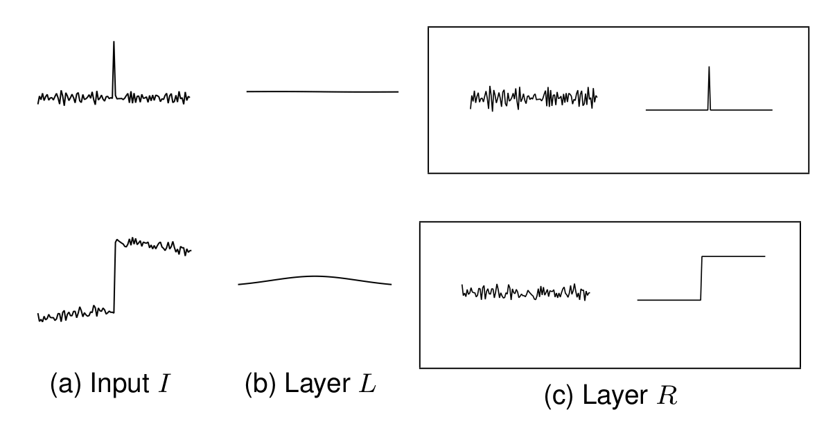
Figure 2. The 1-D signal ${I}$ is decomposed into three basic components: a spatial-varying ${L}$, a detail texture layer and a salient edge. We attribute the texture and edge into the reflectance ${R}$ in our intrinsic image model.

Recall the spatial-varying illumination, we have $s^l_k \approx \bar{s^l_k}$ with mean value $\bar{s^l_k}$ in local patch ${k}$. Besides, if two patches ${i}$ and ${j}$ are close to each other, we also have $\bar{s^l_i} \approx \bar{s^l_j}$. As shown in Figure 2, the two claims are valid in both flat regions (Top) and strong edges (Bottom). Substituting them into Eq. (\ref{eq:eq7}) we can further simplify the “encoding” model into,

\[\begin{equation} \label{eq:eq9} \begin{aligned} {s}_{i} &=({s}^{r}_{i}+s^l_i) \approx ({s}^{r}_{i}+\bar{s^l_i}) = ({\sum\nolimits_{j \in \Omega_{i}}{\omega_{i,j}^{s^r}}s^r_j}+\bar{s^l_i}) \\ &= \sum\nolimits_{j \in \Omega_{i}}{\omega_{i,j}^{s^r}}(s^r_j+\bar{s^l_i}) \approx \sum\nolimits_{j \in \Omega_{i}}{\omega_{i,j}^{s^r}}(s^r_j+\bar{s^l_j}) \\ &\approx \sum\nolimits_{j \in \Omega_{i}}{\omega_{i,j}^{s^r}}(s^r_j+s^l_j)=\sum\nolimits_{j \in \Omega_{i}}{\omega_{i,j}^{s^r}}{s_j}. \end{aligned} \end{equation}\]

As we can see, Eq. (\ref{eq:eq9}) and (\ref{eq:eq7}) have the same form and ${\omega_{i,j}^{s^r}}$ keeps invariant when adding a constant illumination ${\bar{s^l_i}}$ back. Due to the translation-invariant property of local linear model, the reflectance layer can be directly regularized without the necessity of decoupling the reflectance from an image. Putting Eq. (\ref{eq:eq7}) and (9) into Eq. (\ref{eq:eq8}), we have reflectance loss ${E^r(o)}$,

\[\begin{equation} \label{eq:eq10} \begin{aligned} &E^r(o)={\sum_{i} {(o_i-{\sum_{j \in \Omega_{i}}{\omega_{i,j}^{o}}{o_j}})}^2}\\ \text{s.t.}&\quad {\omega_{i,j}^{o}}= {\omega_{i,j}^{s}}, \quad {s_i}= \sum_{j \in \Omega_{i}}{\omega_{i,j}^s s_j}, \end{aligned} \end{equation}\]

where ${\omega_{i,j}^{s}}={\omega_{i,j}^{s^r}}$ and ${\omega_{i,j}^{o}}={\omega_{i,j}^{o^r}}$ for local “encoding” weights. The relationship between Eq. (\ref{eq:eq8}) and Eq. (\ref{eq:eq10}) is clear, as the first constraint in Eq. (\ref{eq:eq8}) is chosen as the objective function and the others act as constraints. As we can see, Eq.(\ref{eq:eq10}) contributes an identical regularizing role as Eq. (\ref{eq:eq6}). The simplification roots in the translation-invariant property of locally linear embedding (LLE), which helps to faithfully penalty non-consistent structures despite the local illumination deviation between the input and exemplar images. Moreover, this reduction enables us to translate the reflectance layer from the source illumination surface to that of the exemplar, while keeping the reflectance layer from changing.

Content loss:

We additionally introduce a so-called content loss to avoid the illumination over-fitting problem, which may occur when the pre-computed examplar has a strong over-stretched illumination. The content loss, in such cases, helps to give a remedy for the output global illumination. Specifically, we define the content loss ${E^c(o)}$ as,

\[\begin{equation} \label{eq:eq11} \begin{aligned} E^c(o)&=\sum_{i} {(o_i-s_i)}^2. \end{aligned} \end{equation}\]

We can verify that Eq.(\ref{eq:eq11}) is essentially defined on the illumination layers. We also have ${E^c(o)=\sum_{i} (o_i^l-o_i^r+s_i^l-s_i^r)^2=\sum_{i} (o_i^l-s_i^l)^2}$ with ${o_i^r} = {s_i^r}$ under the illumination-invariant property of the reflectance layer. It is valuable to note that ${E^c(o)}$ is not always necessary but plays an auxiliary role to prevent output illumination from being over-dependent on exemplars.

Optimization

Now, we combine three loss functions and rewrite Eq. (\ref{eq:eq12}) in a matrix form:

\[\begin{equation} \label{eq:eq12} \begin{aligned} E(o) =&\alpha {\left\Vert K^o o-K^c c \right\Vert}_2^2+\beta{\left\Vert M o \right\Vert }_2^2+\gamma{\left\Vert \boldsymbol{o-s}\right\Vert }_2^2, \\ &\text{s.t.} \quad \omega_{i,j}^{o}= {\omega_{i,j}^s}, \quad {s_i}= {\sum_{j \in \Omega_{i}}\omega_{i,j}^{s} s_j}, \end{aligned} \end{equation}\]

where ${K^{o}(K^{c})}$ is a kernel affinity matrix, whose ${(i,j)}$th entry is ${K_{i,j}^{o(c)}}$; and ${M=[I-W]}$ is a sparse coefficient matrix with identity ${I}$ and weight ${W}$ containing entries ${\omega_{i,j}^{o}}$. Once ${K^o}$, ${K^c}$ and ${W}$ are pre-computed, the output image can be reconstructed by solving the Eq. (\ref{eq:eq12}) directly.

We first compute the filter kernel ${K}$. The simplest case can be the ${2}$-D Gaussian filter (GF), where ${f}$ relies on pixel’s position: ${p=[p_x, p_y]}$ with the ${x}$ and ${y}$ directional coordinates ${p_x}$ and ${p_y}$ respectively. One can use bilateral filter (BF) for more robust results, which considers both the pixel’s position ${p=[p_x, p_y]}$ and color intensities $(R_i,G_i,B_i)$.
We set ${\delta_{f_i}=\delta_s}$ for the Gaussian filter and ${\delta_{f_i}=(\delta_s,\delta_r)}$ for the bilateral filter. For simplicity, we set ${K =K^o=K^c}$ in our experiments due to the unavailable of the image $o$ in advance.

For the LLE weights, it may be unstable to take a direct solver, when the number of neighbors of each point is larger than the space dimension. As described in, a remedy ${W}$ can be computed by solving the point-wise regularized problem,

\[\begin{equation} \label{eq:eq13} \begin{aligned} \min{\sum_i ({s_i}-{\sum_{j \in \Omega_i}{\omega_{i,j}^{s} {s_j}}})^2}+\epsilon {\Vert \omega^s\Vert}_2^2, \text{s.t.} \sum_{j \in \Omega_{i}} {\omega_{i,j}^{s}}=1. \end{aligned} \end{equation}\]

We refer the reader to some more complex regularizers such as the modified LLE algorithm, in which more robust solutions are given to distribute the contribution of neighbours to each point more uniformly.

After obtaining the ${K}$ and ${W}$, Eq. (\ref{eq:eq12}) can be solved by setting ${dE/do=0}$, giving the following linear system: $\begin{equation} \label{eq:eq14} \begin{aligned} (\alpha K^{T} K + \beta M^{T} M +\gamma I) o=\alpha K^T K c + \gamma s, \end{aligned} \end{equation}$

where ${L =\alpha K^T K + \beta M^T M +\gamma I}$ is a large-scale and sparse {Laplacian matrix}. Since ${L}$ is symmetric and semi-positive, Eq. (\ref{eq:eq14}) can be solved with the solvers such as Gauss-Seidel method and preconditioned conjugate gradients (PCG) method.

In summary, our IIT algorithm includes: identifying the filter kernel for illumination fitting, computing LLE weights to encode image reflectance, and embedding the reflectance layer for image reconstruction. The whole minimization scheme is presented in Algorithm 1.

Experimental Results

We verify the proposed IIT model with the aid of an extra “exemplar” image. As explained, our model may require a latent illumination layer in the sense that the underlying target illumination in many illumination-related tasks could deviate greatly from that of the original image. Nevertheless, it is not easy to provide such an illumination layer because of the inherent intractability of intrinsic image decomposition. Alternatively, we introduce a pre-computed “exemplar” and use it to provide the underlying illumination approximately. Notice that, we specify the fine-balanced illumination distribution of the exemplar, but the proposed IIT framework does not rely on any specified exemplars.

We take two representative exemplars into account to verify the easy-fulfilled requirements of the exemplar and its benefits to image illumination manipulation. The first class of exemplars is generated by the simple TMO methods — for example, contrast limited adaptive histogram equalization (CLAHE) method which provides an exemplar with fine-balanced illumination distribution but distorted local details. The second class of exemplars is given by the existing cutting-edge methods, which usually provide an exemplar exhibiting better quality with not so strong local artifacts as the CLAHE ones. They are selected in consideration of the different properties in color, saturation, textures, noises, and illumination conditions.

Verification and Robustness:

Firstly, we show the results with a CLAHE exemplar. As shown in Figure 3, the exemplar in Figure 3b is generated by the CLAHE algorithm with the fine-balanced illumination but distorted local details, while our IIT algorithm exhibits significant improvements in suppressing the local noises and distortions, especially around the swan’s “neck” and “wing” regions in Figure 3c and Figure 3d. Moreover, tiny visual differences occur between using the Gaussian and bilateral filters.

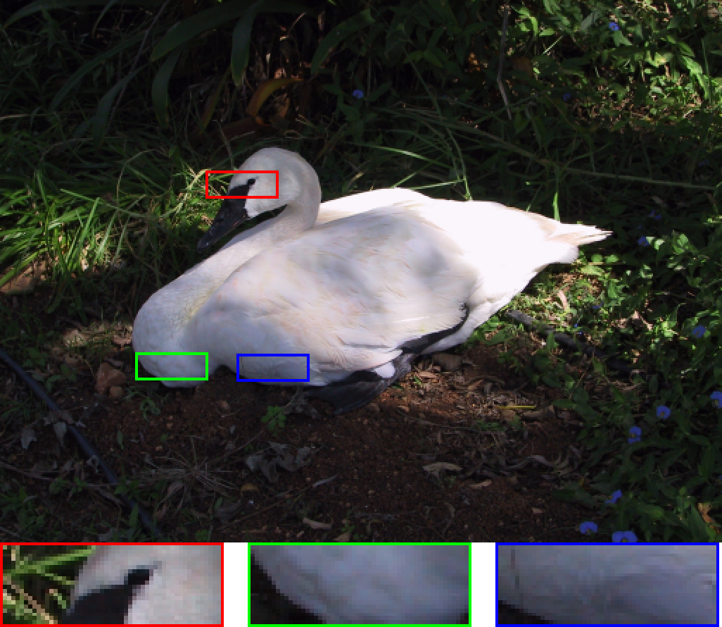
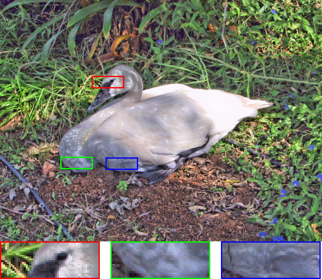
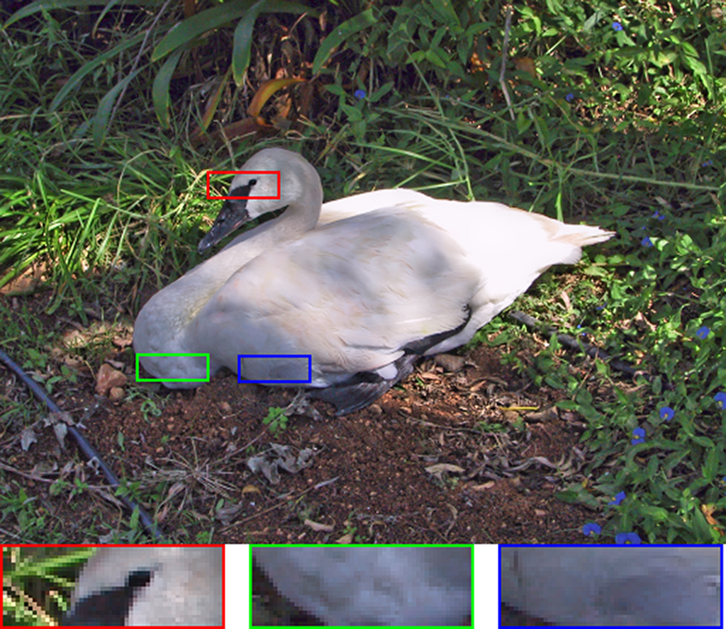
Figure 3. Visual results of our IIT algorithm with the Gaussian and bilateral filters, respectively. (a) Source, (b) CLAHE exemplar, (c) and (d) Our results. The noise and distortions are suppressed significantly in comparison to the CLAHE exemplar. TMQI (b)-(d): 0.845, 0.891, 0.898.

We further explain the ability of our IIT method in fitting the latent image illumination determined by the exemplars. As shown in Figure 4, we present two typical exemplars given by the CLAHE algorithm. The exemplars in Figure 4b and Figure 4d should have different underlying illumination, as they exhibit different levels of brightness regardless of the slight texture distortions. In this case, we set $\alpha \!=\! 1.0$ and $\gamma \!= \!0$ to enforce the output be close to the exemplar. It is noticeable that the outputs in Figure 4c and Figure 4e reveal identical illumination distribution as that of the exemplars, and the non-consistent details in the exemplars are significantly suppressed in both cases. The results prove that a balanced image illumination instead of high-quality local details is the key ingredient to our IIT method. This observation is consistent with the assumption that the exemplar plays a determining role in improving the balance of image illumination, while local textures have little contribution to the output illumination.

Figure 4. Visual comparison of our IIT algorithm by using exemplars with different levels of brightness. (a) Input image; (b) and (d) CLAHE exemplars; (c) and (e) our IIT results.

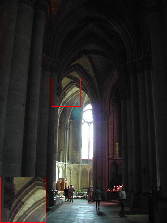
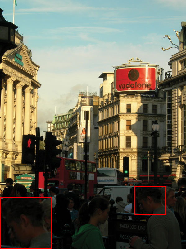
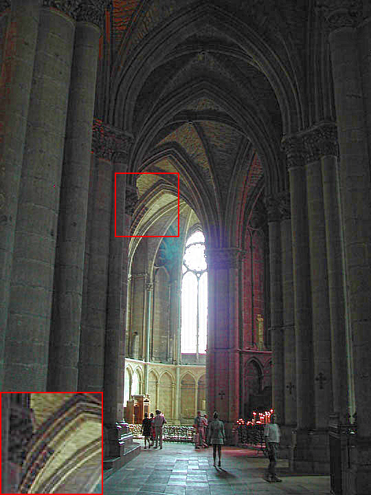
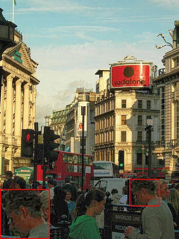
We additionally illustrate the robustness of our IIT method to the exemplar with strong local degraded details. As shown in Figure 5, we interpret the illumination compensation results on Yale Face dataset. In this case, two typical exemplars (b) and (d) are introduced to show the robustness of our method to noise (Top) and textural distortions (Bottom). In the top row, the exemplars are cropped with different levels of Gaussian noise; while, in the bottom row, the exemplars suffer from serious textural distortions given by the CLAHE algorithm\footnote{As interpreted in CLAHE, we set the “NumTiles = ${16\times16}$” and “NumTiles = ${32\times32}$” for the exemplars in Figure 5b and Figure 5d, respectively. A larger “NumTiles” leads to stronger textural distortions.}. Again, our IIT method produces the satisfying results Figure 5c andFigure 5e that have identical illumination distribution as the exemplars, but the non-consistent textures are significantly suppressed, especially in “face” regions. Moreover, the quality of outputs only drops slightly if we only increase the level of textural distortions but keep the illumination distribution invariant.

Figure 5. Illumination compensation on Yale Face dataset. (a) Source, (b) and (d) CLAHE exemplars, (c) and (e) results (IIT+ BF). TMQI, top: 0.935, 0.985, 0.833, 0.981; bottom: 0.922, 0.967, 0.897, 0.965.

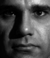
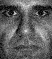
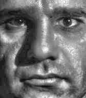
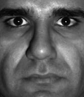
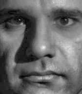
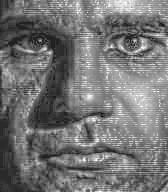
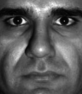
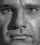
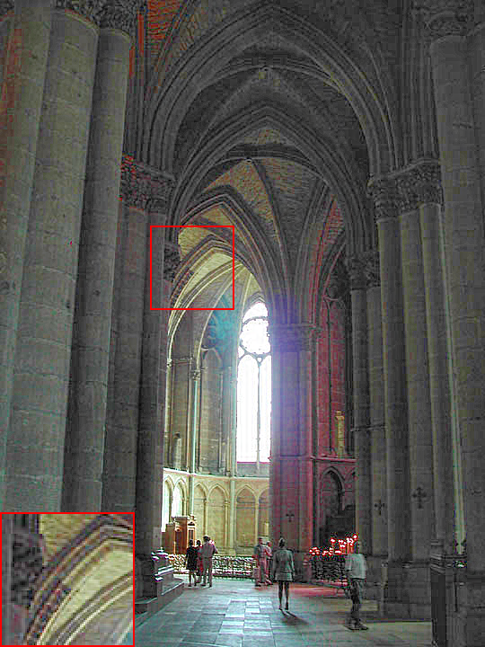
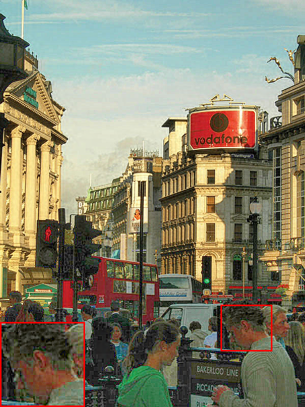
The above experimental results imply that image illumination can be faithfully controlled with the aid of an “exemplar”, because there is no need to pay much attention to local distortions and artifacts. As a result, it is easy to obtain a suitable exemplar by using many existing methods. This advantage is mainly beneficial from the use of the smoothing operator in illumination loss and the translation-invariant property of the LLE “encoding” model. On the one hand, the local details are mostly filtered out by the smoothing filter in the illumination loss, which remarkably weakens the impact of textural distortions; on the other hand, the inaccuracy of the smoothed illumination would be further corrected by the LLE “encoding” model. The two aspects help to penalize the non-consistent structures existing in the exemplar significantly, thereby giving a practical way to reconstruct natural-looking results with high-quality consistent local details.

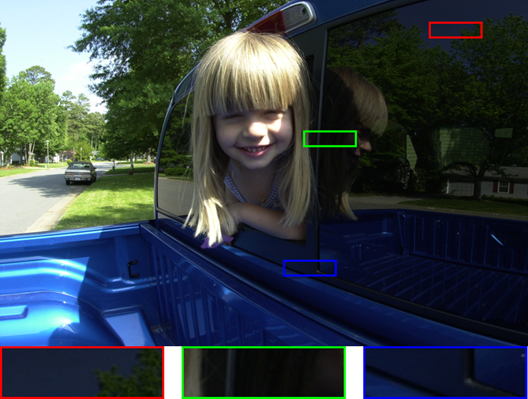
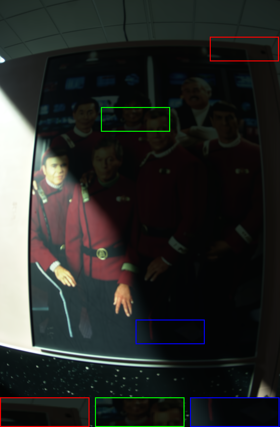
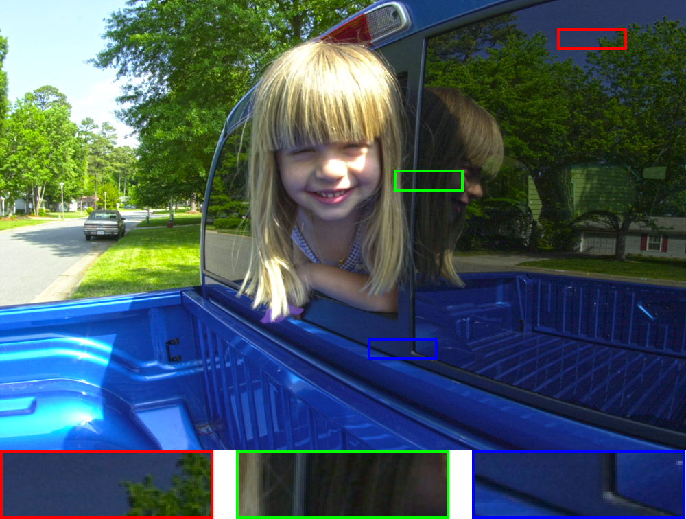
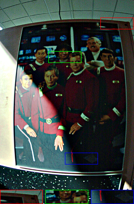
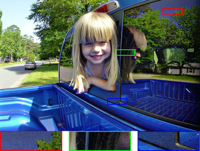
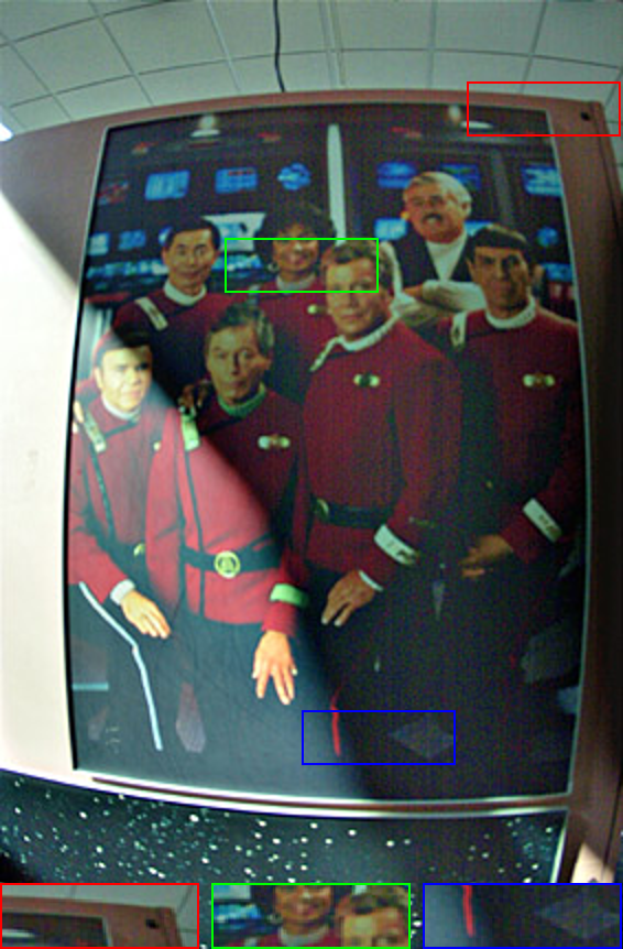
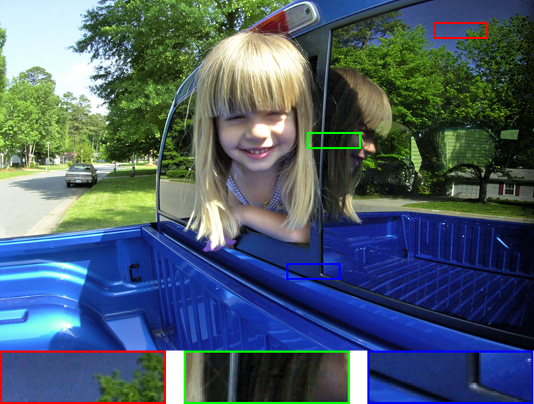
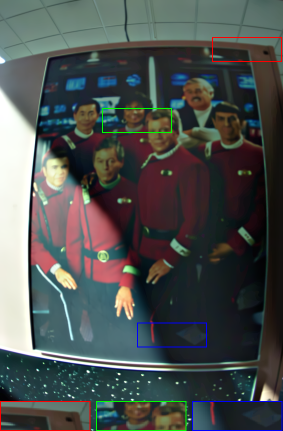
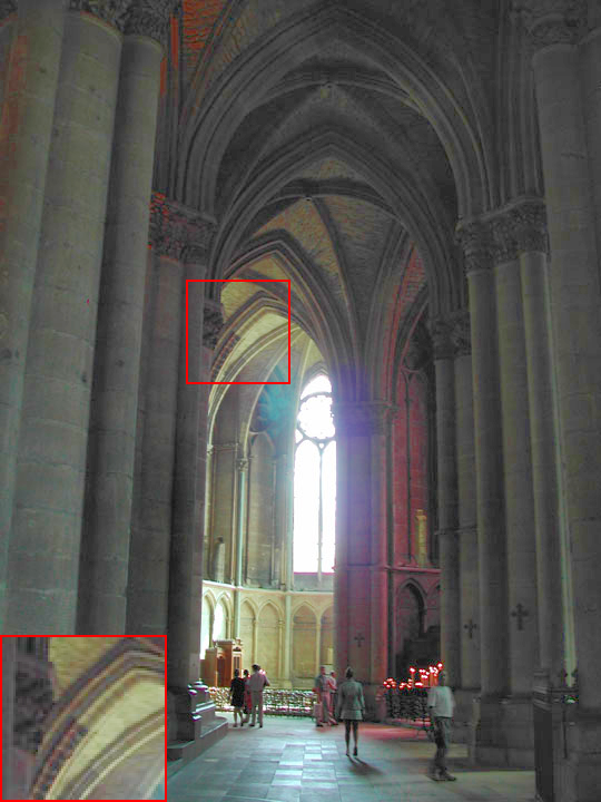
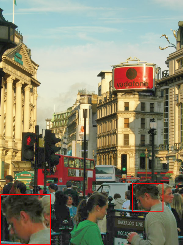
Figure 6. Visual comparison of image enhancement. The exemplars in (c) are produced by the state-of-art NASA Retinex. TMQI, top (b)-(d): 919, 0.943, 0.946; and bottom (b)-(d): 0.922, 0.916, 0.944.

Secondly, we validate our IIT algorithm with an exemplar given by the state-of-the-art. In general, they produce an exemplar with much better quality than that of the CLAHE method. We adopt the default configurations or preferable parameter-settings as suggested in these methods. We set ${\alpha, \beta}$ and ${\gamma}$ to 0.95, $[10, 100]$ and 0.05, respectively, and the parameter $\beta$ may vary according to the level of artifacts existing in exemplars. We let ${\alpha \gg \gamma}$ in view of the balanced illumination distribution of the exemplars. 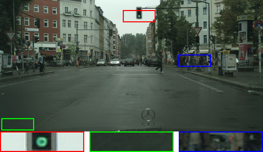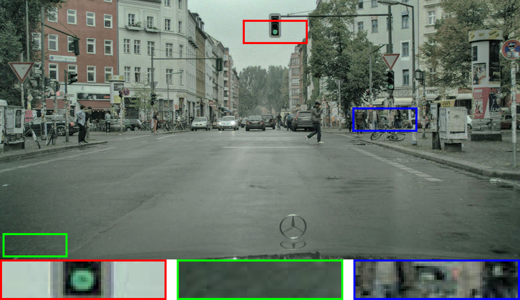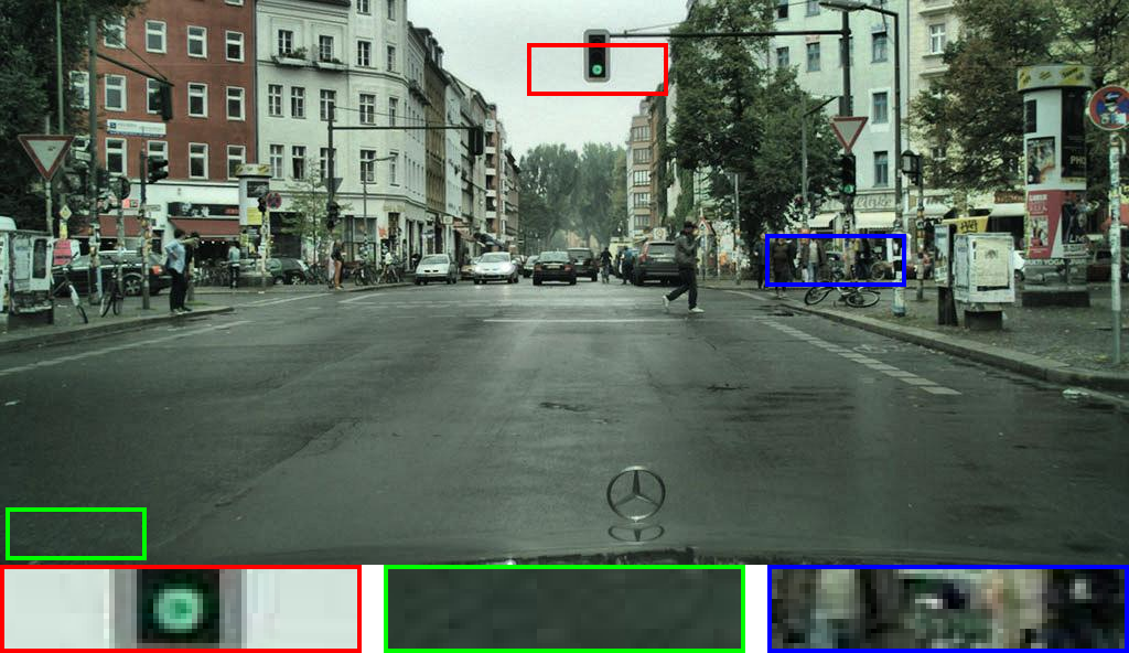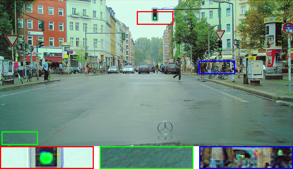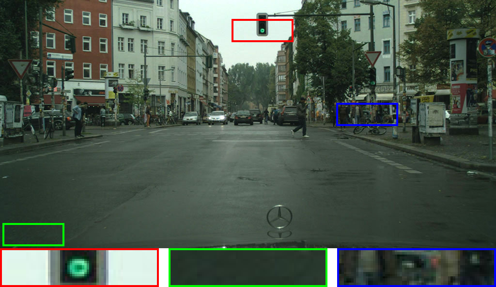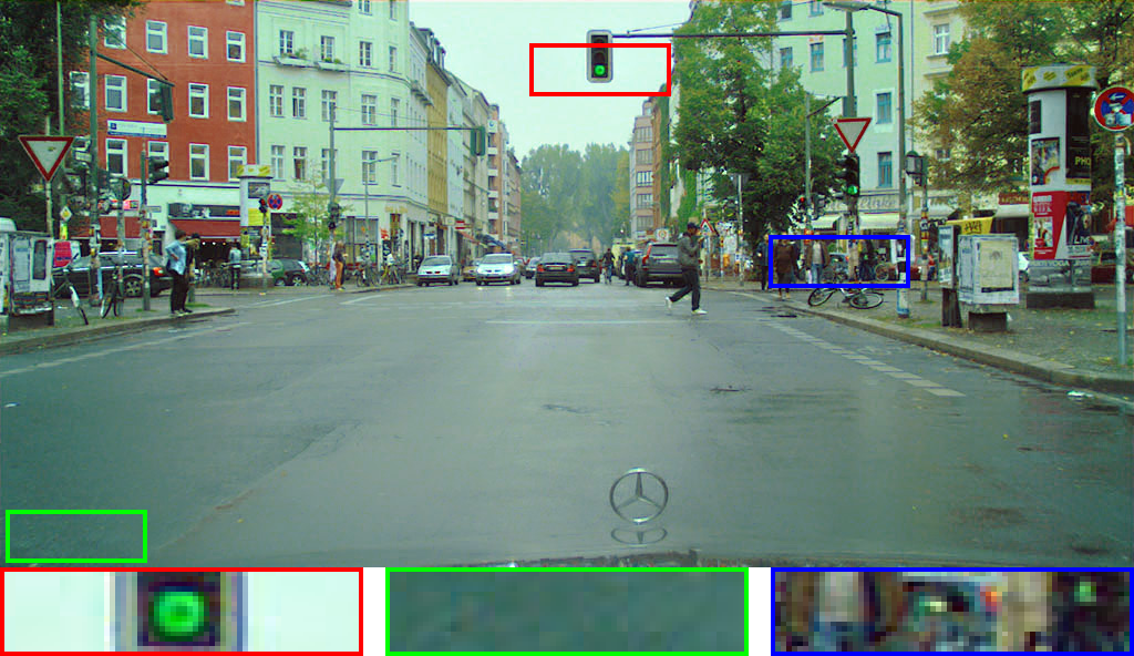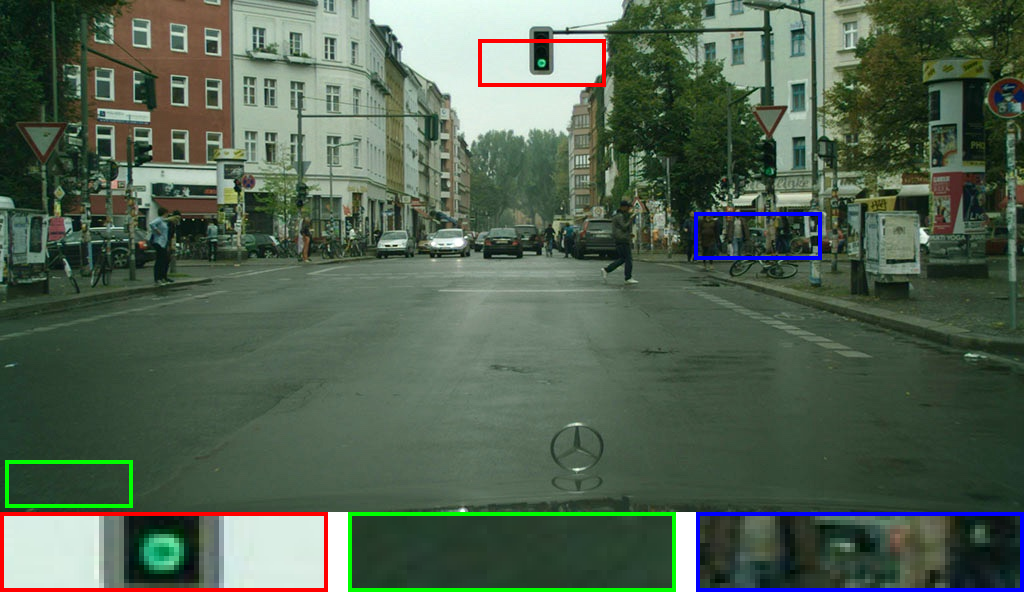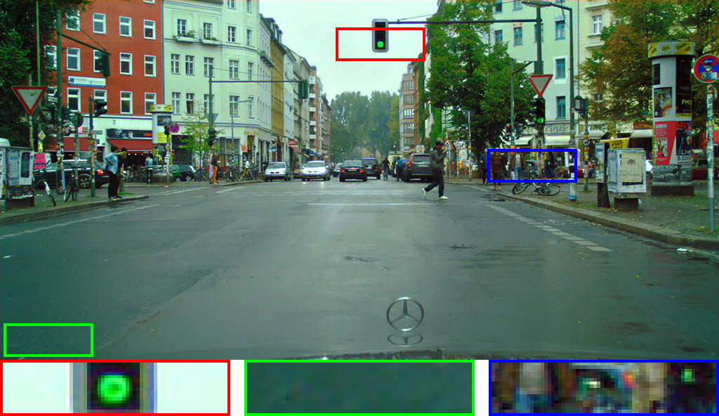As shown in Figure 6, we compare the results with the Photoshop CC and NASA Retinex methods, where the exemplars are provided by the cutting-edge NASA Retinex. It is notable that Photoshop CC gives the results with limited improvement in dark regions based on the built-in “HDR tone mapping” tool, while the NASA Retinex method produces high-quality results with vivid color and contrast but also suffers from strong noise. In contrast, our IIT method attains similar enhanced results as the NASA Retinex with more consistent local textures compared with Photoshop CC and NASA Retinex results.

Figure 7. Visual comparison on Cityscapes dataset. The exemplars used in (g) and (h) are given by the state-of-art (f) WESPE. TMQI, (b)-(h): 0.891, 0.913, 0.973, 0.893, 0.801, 0.921, 0.942.

The result is further demonstrated on the Cityscapes dataset, in which the images suffer from visible degradation in color, saturation, and textures due to the low resolution and inappropriate illumination conditions. In this situation, it is often difficult for many existing methods to recover high-quality results. As shown in Figure 7, the prevailing commercial software, including Google Nik (GN), Apple Photo Enhancer (APE) and Adobe Photoshop CC 2018 also reveal drawbacks in producing natural-looking results, where the automatic parameter-settings are adopted for comparison. Recent deep-learning approaches such as WESPE provide a solution to visual-pleasant results, but there still exists some unpleasant artifacts such as over-exaggerated details around the salient edges. In contrast, our IIT method can be applied to correct these artifacts for high-quality consistent local details. As we can see in Figure 7g and Figure 7h, we take the WESPE result as the exemplar and the local structures of “street lamp” are precisely preserved and the “road” reveals little texture distortions compared with the other methods.

We now have investigated the role of exemplars in our IIT method and demonstrated the robustness to produce high-quality results under different types of exemplars. We also conclude that many existing methods can be used to provide such an exemplar. As interpreted before, the whole procedure, with the aid of an exemplar, is eventually formulated into a generalized optimization framework, giving a closed-form solution to a wide range of illumination-related tasks. The favorable results definitively benefit from both the smoothing operators in illumination loss — which helps to reduce the impact of local details in the exemplar, and the LLE encode in reflectance loss — which adaptively extracts local details from the original image and then embeds them onto a new smoothing surface given by the exemplar. The merit is the use of an exemplar, which significantly simplifies image illumination manipulation because of avoiding an explicit intrinsic image decomposition.

Quantitative Evaluation:

In this section, we further take a quantitative evaluation based on the following datasets: Cityscapes, NASA Retinex and DPED. The Cityscapes dataset has 20 low-resolution images with slightly unbalanced illumination distribution, which are challenging for many existing methods; while NASA Retinex and DPED datasets have 26 and 16 images respectively, which have higher resolution but also reveals strong imbalance illumination distribution. The proposed IIT method is compared with the cutting-edge methods, including NASA Retinex, Google Nik (GN), Apple Photo Enhancer (APE), Adobe Photoshop CC 2018, WESPE method, and the exemplars in the datasets are provided by the Retinex, WESPE and CLAHE methods, respectively.

Table 1. Quantitative evaluation on Cityscapes, NASA Retinex, and DPED datasets. The exemplars in the datasets are given by the WESPE, Retinex, and CLAHE methods, respectively.
Method	(SF / SN) TMQI	IL-NIQE	NIMA	(SF / SN) TMQI	IL-NIQE	NAMA	(SF / SN) TMQI	IL-NIQE	NIMA
	Cityscapes (WESPE)			NASA (Retinex)			DPED (CLAHE)
NASA Retinex	(- / -) -	-	-	(0.916 / 0.731) 0.937	20.71	4.562	(- / -) -	-	-
Photoshop CC	(0.988 / 0.323) 0.887	17.37	3.859	(0.948 / 0.428) 0.892	21.65	4.003	(0.982 / 0.507) 0.916	22.38	4.479
APE	(0.946 / 0.272) 0.840	24.25	4.002	(0.981 / 0.618) 0.937	20.91	3.922	(0.980 / 0.566) 0.927	21.62	4.613
Google Nik	(0.927 / 0.527) 0.906	21.32	4.131	(0.968 / 0.812) 0.965	23.15	3.822	(0.963 / 0.567) 0.925	21.53	4.523
WESPE	(0.915 / 0.839) 0.956	20.25	4.338	(- / -) -	-	-	(0.931 / 0.626) 0.928	22.25	4.534
IIT+GF (Ours)	(0.979 / 0.835) 0.971	4.252	4.313	(0.957 / 0.650) 0.936	20.62	4.475	(0.969 / 0.587) 0.929	21.95	4.555
IIT+BF (Ours)	(0.981 / 0.826) 0.970	16.48	4.293	(0.960 / 0.678) 0.942	20.57	4.470	(0.973 / 0.589) 0.931	21.31	4.540

In general, image quality assessment can be categorized into full-reference and no-reference approaches. The full-reference methods always require the corresponding ground-truth images for high-accuracy assessment, which, however, are always not available in the case of illumination-related tasks. As a result, it is difficult to take an objective full-reference evaluation. In contrast, no-reference methods require no ground-truth images but rely on statistical models to measure the degradation of an image. Recent no-reference approaches, in particular these deep-learning ones, have also shown promising success in predicting the quality of images. Specifically, we employ a quantitative evaluation based on the Tone Mapped Image Quality Index (TMQI), Integrated Local Natural Image Quality Evaluator (IL-NIQE) and Neural Image Assessment (NIMA). The TMQI index is a full-reference image assessment method built on the source and output images, which is originally proposed to provide an objective image quality assessment for HDR image compression. In TMQI index, Structural Fidelity (SF) and Statistical Naturalness (SN) are considered to provide an objective quality assessment. The SF index is based on the multi-scale structural similarity (SSIM) approach to extract structural information from the visual scene and provides a perceptual predictor of structural fidelity. The SN index provides a statistic metric for the output image, which takes the natural image statistics of brightness, contrast, visibility and details into account. IL-NIQE and NIMA are two no-reference image assessments. The former is a learning method based on natural image statistics features derived from color, luminance, gradient and structure information; and the latter attempts to predict consistent aesthetic scores with human opinions using convolutional neural networks. The NIMA method is trained on a large-scale natural image dataset for perceptually-aware no-reference quality assessment. The statistical results are shown in \textbf{Table} \ref{tab:tab1}, where the best two results are highlighted with \textbf{bold} and \textbf{underline}, respectively. The advantage of our IIT method is noticeable with 19 top-two places in total 30 indices compared with the state-of-art on real-world image datasets.

More Extensions

It is easy to see the proposed IIT method can be extended to high dynamic range (HDR) image compression to improve the visibility of dark regions. Similarly, it helps to suppress the distorted details or artifacts, providing the comparable or superior results than the prevailing cutting-edge methods. In this case, we apply the proposed IIT model on image luminance with the same aforementioned configurations. The saturation is restored with a heuristic de-saturation setup as described in.

\[\begin{equation} \begin{aligned} C_{out}={\left(\frac{C_{in}} {L_{in}}\right)}^s L_{out}, \end{aligned} \label{f2} \end{equation}\]

where $C =\{ R,G,B\}$ are red, green and blue channels of color images, $L_{in}$ and $L_{out}$ denote the source and mapped luminance, and $s$ controls the saturation with an empirical value between 0.4 and 0.6 to produce satisfying results.

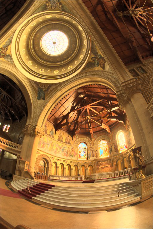
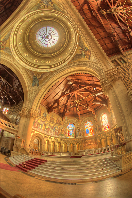
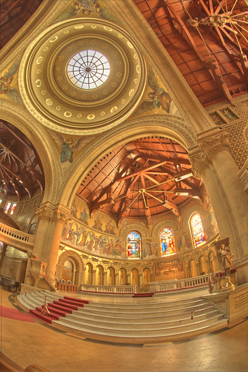
We show two examples of HDR image compression with visual comparisons in Figure 8, where the exemplars are generated by the CLAHE algorithm. We set the parameter $s = 0.5$ and $s=0.6$ for the two cases, respectively. As we can see, the proposed IIT method is capable of producing high-quality results as that of the gradient-domain (GD) compression and weighted least square (WLS) filtering method.

Figure 8. Visual comparison of the HDR image compression using the CLAHE exemplars. TMQI, top (a)-(c): 0.923, 0.948, 0.944; bottom (d)-(f): 0.912, 0.940, 0.953.

We additionally illustrate that the structure-consistent property of the proposed IIT method makes it applicable to much more complex situations beyond the above illumination-related tasks. Specifically, it is possible to be used as a building block for color transform and style transfer, where a high-level vision image-to-image translation is always deduced to produce stylized results for artistic purpose. In the literature, many approaches, especially the deep-learning ones, have been explored to obtain artistic-like stylized results. Despite their great success, they occasionally produce unexpected distortions or unrealistic artifacts that not occur in real photographs. We illustrate that the proposed IIT model is possible to suppress these non-consistent textures, enjoying a photo-realistic style transfer as proposed in the recent work. The understanding for style transfer, somewhat, remains elusive and the discussion for more details is out of scope here, we conjecture here that the image-to-image translation procedure can be also interpreted under the intrinsic images of Eq. (\ref{eq:eq1}). The difference from the illumination-related works is that both illumination and reflectance layers in style transfer vary significantly, leading to a strong discrepancy in image color, saturation, texture, style, and so on.

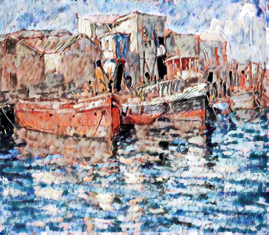
We briefly illustrate the procedure by giving an input image and a reference style, where a stylized exemplar is firstly generated by the existing style transfer methods such as the deep learning ones. Our IIT algorithm is then used to refine the local distortions of the stylized exemplar. As shown in Figure 9, an image Figure 9a is first transformed into the stylized exemplar Figure 9c using two deep learning-based methods under the guidance of reference style Figure 9d; and a photo-realistic result Figure 9b is obtained under the IIT model with the stylized image as the corresponding exemplar. As we can see, our IIT algorithm produces satisfying results that have identical saturation as the exemplar and high-quality consistent structures as the input image. The local textures in the “sky” region are remarkably removed, leading to the photo-realistic stylized results. The startling results demonstrate the powerful ability of the proposed IIT method in suppressing the local distortions, and it further turns out the robustness of our method to the exemplar image.

Figure 9. Photorealistic style transfer. Given an image (a) and a reference style (d), a stylized exemplar (c) may be provided by these deep-learning methods, which is further refined by our IIT model as shown in (b) with more consistent textures and structures.

Conclusion

This paper has described an intrinsic image transfer algorithm, which is rather different from recent trends towards making an intrinsic image decomposition. This model creates a local image translation between two image surfaces and produces high-quality results in a wide range of illumination manipulation tasks. One drawback is that the algorithm is time-consuming for the need of computing the large-scale LLE weights and PCG solver. It is possible to be addressed with a sub-sampling strategy for efficiency, which is left for future work.